|

Eng.cam.ac.uk

Real Options: Competition in Market Regulation and Cooperation in Partnership Deals Judge Business School Fitzwilliam College, University of Cambridge A thesis submitted for the degree of Doctor of Philosophy To my family, for their unconditional love and support.
This thesis is a collection of four papers. The first three papers are written for an academic audience, while the fourth paper is written with a mixed audience of academics and managers in mind.
The paper in Chapter 2 is one of the outcomes of collaborative work with Fa- bien Roques. I was responsible for the development of models and their analytical and numerical solution, whilst Fabien contributed his expertise in electricity mar- kets regulation. The collaboration resulted in two working papers, one of them has an electricity regulation focus and is available as a Cambridge Working Paper in Economics. The paper included in this thesis has been written by myself and is largely a summary of my own contribution to the collaboration. In view of the collaboration, Fabien Roques should be regarded as the second author of this paper. I would quantify his contribution as 20% of the paper.
The paper in Chapter 4 is part of ongoing joint work with my supervisor Ste- fan Scholtes. I was responsible for the development of the model and its analysis.
The structuring of the paper was done jointly. Stefan Scholtes is the second au- thor of this paper. I would quantify his contribution as 20% of the paper.
The papers in Chapter 3 and Chapter 5 are entirely my own work and in- clude nothing which is the outcome of work done in collaboration, except where specifically indicated in the text.
I am grateful to my PhD supervisor Stefan Scholtes who never failed to provide valuable help and support, far beyond the formal supervi- sor requirements. Working with him has been inspirational. I hope to prove worthy of the trust he has shown in me.
I would also like to thank the Cambridge Commonwealth Trust for partially funding my studies through a bursary.
Real Options: Competition in Market Regulation and Cooperation in Partnership Judge Business School Fitzwilliam College, University of Cambridge A thesis submitted for the degree of Doctor of Philosophy This thesis is a contribution to the field of investment under uncertainty. We develop two new application areas of significant practical importance: regulatory intervention and cooperation. The thesis consists of two related but stand-alone The first part investigates the effect of regulatory intervention in the form of a price cap in an oligopolistic market with irreversible investment under uncertainty.
We find that there is a trade-off between the beneficial effect of regulation on preventing anticompetitive behaviour and the detrimental effect of destroying incentives for investment in new capacity. Our contribution is to solve the problem for an oligopolistic market with time-to-build. Interestingly, the introduction of price cap regulation, when it takes time to build new capacity, results in three locally stationary strategies. This multiplicity of solutions has, to the best of our knowledge, not been observed before in similar real options models.
The second part of the thesis examines real options in projects developed in partnerships. We present a formal framework, borrowing ideas from cooperative game theory and efficient risk sharing, to address real options in partnerships.
We conclude the second part of the thesis with an account of a recent R&D partnership in the biopharmaceutical sector. We identify examples of seemingly sensible deal structures that lead to surprising and somewhat counterintuitive results in the presence of uncertainty.
Technical literature . . . . . . . . . . . . .
Investment under uncertainty with price ceilings Model assumptions . . . . . . . . . . .
Nash-Cournot equilibrium investment strategies . . .
Impact of price ceiling regulation . . . . . . . . .
Nash-Cournot equilibrium with a price cap . . . . .
Sensitivity analysis and simulations . . . . . . . . .
Price cap effectiveness . . . . . . . . . .
Robustness of price cap regulation . . . . . . .
Trade-off between robustness and effectiveness .
Market evolution and the long term effect of price regulation Simulation parameters . . . . . . . .
Market evolution . . . . . . . . .
Impact of price cap on capacity installed . . .
Impact of price cap on long term average price Price ceilings with time-to-build Investment price trigger Asymptotic behavior of investment price trigger . . .
Time lag tends to zero . . . . . . . .
Price cap tends to infinity . . . . . . .
Investigation of investment price trigger Equilibrium investment of a symmetric oligopoly . . . . .
Trade off between price cap effectiveness and robustness Simulation of regulated market with time-to-build . . .
Appendix 1: proof of proposition . . . . . . .
Appendix 2: calculating Z(P) . . . . . . . .
Appendix 3: proof of propositions and . . . .
Real options in partnerships Options contracts: cooperative vs. non-cooperative options . .
The core of an options contract: an illustrative model . . . .
The core of the deterministic game . . . . . . .
Uncertain payoffs . . . . . . . . . . . .
Complete markets . . . . . . . . . . . .
The contract without options . . . . . .
A cooperative option . . . . . . . .
A non-cooperative option . . . . . . . No traded assets and risk-neutral agents . . . . . The non-cooperative option . . . . . . Cooperative games and risk aversion . . . . . . Cooperative options and risk aversion . . . . . . Non-cooperative options . . . . . . . . . . Cooperative real options games in continuous-time . . . . . Cooperative options in complete markets . . . . . Unilateral options in complete markets . . . . . . Risk aversion in the absence of hedging opportunities . . Non-cooperative options and risk aversion . . . . . Managerial implications and conclusions . . . . . . . A R&D deal in the biotechnology sector A R&D alliance in the biotechnology sector The drug research and development process . . . . Cambridge Antibody Technology . . . . . . . A framework for analyzing partnership deals in the biotechnology Effect of uncertainty on R&M contracts Contracts with flexibility and the effect of uncertainty . . . . Co-development with an opt-out clause . . . . . . Portfolio effects and organisational issues . . . . . . . Enabling exercise of flexibility . . . . . . . . Conclusions and managerial implications . . . . . . . Price trigger vs. market concentration Investment price trigger vs. price cap for N = 2, 4 . . . . .
Optimal price cap vs. demand volatility Maximum effectiveness vs. demand volatility . . . . . .
Robustness vs. effectiveness . . . . . . . . . . .
Base case simulation parameters . . . . . . . . . .
Price and capacity evolution for one demand realisation . . .
Average installed capacity after 10 years (expressed as % of com- petitive market capacity) . . . . . . . . . . . .
Average markup over competitive price after 10 years . . . .
Investment price trigger vs. price cap, θ = 0.5 years . . . .
Investment price trigger vs price cap, θ = 3 years Value of the firm vs. price cap . . . . . . . . . .
Investment price trigger at different levels of competition . . .
Globally optimal investment price trigger vs. price cap . . .
Globally optimal investment price trigger vs. price cap . . .
The trade-off between price cap effectiveness vs robustness . .
simulation results . . . . . . . . . . . . . .
The core of the cooperative game with the biotech having the opt- Decision Tree: Cambridge Antibody and AstraZeneca R&D alli Value of R&M contract vs. uncertainty . . . . . . . . Value of R&M contract vs. royalties . . . . . . . . . Neoclassical economic theory suggests that a firm should invest in a project when its net present value (NPV) is positivThe NPV rule is a good decision tool provided that there is no uncertainty surrounding future cash flows or, alterna- tively, that the investment is completely reversible. However, most investment decisions involve both a significant amount of uncertainty as well as investment irreversibility. Implicitly, the NPV rule assumes that the investment decision is now-or-never, ignoring the fact that most firms have some freedom over the timing and the size of the investment.
By undertaking the investment as soon as the NPV is positive, a firm forgoes the possibility of investing some time in the future. Since future cashflows are uncertain, waiting gives the firm the chance to learn more about the value of the investment opportunity. If the future value declines the prudent firm will not invest, while if the value increases the firm will invest with the reassurance that this is a good investment. This flexibility is valuable because as it caps the downside potential without harming the upside. Of course waiting might be costly, both directly as keeping the option to invest open might come at a cost, as well as indirectly due to the forgone cash flows. However, if there is enough uncertainty the value of flexibility might outweigh its costs.
This alternative way of thinking about investments as options on uncertain cash flow, was developed in the late 1970's by academics working in the field of 1The classic finance text book by for example, includes a chapter on "Making Investment Decisions with the Net Present Value Rule".
finance (for example As the flexibility inherent in many projects resembles financial options, the term real options was coined to describe investment in real Real options theory advocates that investment decisions must be priced in a manner similar to financial options using contingent claims analysis. The ratio- nale behind financial option pricing is that options are redundant assets. Their payoff can be completely replicated by a portfolio of traded assets. In equilibrium there should be no opportunities for arbitrage, therefore the price of the option at any given time should be equal to the price of the traded replicating portfolio. It is also possible to use the replicating portfolio to hedge all risks from purchasing an option, so making investment in financial options risk free. The fact that real options, as opposed to financial options, are written on private assets that are somewhat unique and are not traded creates some complications for real options Several suggestions have been proposed in order to overcome this pro but the debate in the academic community, as well as the practitioner community, is ongoing. One possibility is to assume that the underlying is traded, construct an imaginary replicated portfolio and use it to price the investment opportu- nity. Another possibility is to ignore traded assets all together and use rational expectations and dynamic programming to price the investment opportunity. Al- though this method is internally consistent, it ignores market considerations and hedging opportunities and could potentially mis-price real options. It is worth noting that although the assumptions behind these two methods are quite dif- ferent, under certain conditions they lead to similar results. Hybrid techniques for valuing real options, that explicitly account for both the traded and the non- traded aspect of the underlying uncertainties, have been developed with their own shortcomings (including increased complexity). The approach taken in this thesis is closer to the dynamic programming approach, although it is also amenable to the contingent claims analysis.
1See e.g. 2See for a recent review.
Despite the lack of consensus regarding the exact mechanics and assumptions of pricing real options, real options methodology has proved to be a very useful tool. It is particularly attractive because it explicitly accounts for two important aspects of investment decisions: uncertainty and flexibility. Real options analysis provides a framework for understanding what good managers know anyway: Un- certainty is not necessarily undesirable. Yes it has a negative side, against which management should try to find shelter but it also has an upside that can be very profitable. Effectively, flexibility introduces an asymmetry in the effect of uncer- tainty: it enhances the upside and at the same time it limits the downside. In the twenty years since real options theory was created it has managed to infiltrate a number of disciplines. It is used in fields such as yield management supply chain optimization and strategy It has also started to make an impact on engineering and systems design Most real options theory and application was developed to price investment opportunities for a monopolist acting in isolation or for perfect competition. Un- der this assumption, the real option holder, just like a financial option holder, will base investment decisions only on the price of the underlying asset and does not need to consider any strategic interactions. However, this assumption is often unrealistic. In a number of industries, firms that undertake investments have an impact on market price and thus affect the profits of all firms in the industry.
These firms must base their decisions not only on the stochastic underlying, but also on the actions of other firms in the industry. Recently, progress has been made to extend the real options paradigm to include strategic interactions. A common finding is that the value of real options is eroded by competitive inter- action and that firms are entering more quickly to avoid preemption Since competition causes firms to speed up investment, anticompetitive collu- sion inevitably has something in common with uncertainty: it delays investment.
Of course the reason for the delay is completely different. Uncertainty makes postponement of investment until the price of the stochastic underlying is quite higher than investment costs a prudent strategy. On the other hand, anticompet- itive behavior delays investment in an attempt to gauge prices and reap higher 1.1 Summary of each paper than normal profits. It is not easy for a regulator to decouple the two causes of investment delays. What is worse is that sanctions that aim to curb anticompet- itive behaviour might backfire by destroying investment incentives.
A first theme explored in this thesis deals with real options in regulation. More specifically, we investigate the effect of regulatory intervention in the form of a price cap in an oligopolistic market with irreversible investment under uncertainty.
We find that there is a trade-off between the beneficial effect of regulation on preventing anticompetitive behaviour and the detrimental effect of destroying incentives for investment in new capacity. Our contribution to the theory of regulation under uncertainty is to solve the problem for an oligopolistic market with time-to-build. Interestingly, the introduction of price cap regulation, when it takes time to build new capacity, results in three locally stationary strategies instead of one. This multiplicity of solutions has, to the best of our knowledge, not been observed before in similar real options models.
The second theme of the thesis is real options in partnerships. Traditionally, real options theory is concerned with the valuation of projects with real options owned exclusively by one firm. Frequently, projects are developed by a consortium of firms with different risk profiles and possibly even different strategies. Several interesting questions arise that traditional real options theory cannot answer. For example, how should the partnership structure a contract so that it facilitates a consensus on option exercise strategies? How should they share the value? What is the effect of unilateral flexibility? We present a formal framework, borrowing ideas from cooperative game the- ory and efficient risk sharing, to address real options in partnerships. We con- clude the second part of the thesis with an account of a recent R&D partnership in the biopharmaceutical sector. We identify examples of seemingly sensible deal structures that lead to surprising and somewhat counterintuitive results in the presence of uncertainty.
Summary of each paper We now discuss each part in more detail.
Part I: Real Options and Competition in Market Regulation.
1.1 Summary of each paper Chapter 2: Intertemporal price cap regulation and incentives to invest in new capacity. The first chapter of Part I of the thesis investigates the effect of price cap regulation on investment in new capacity at different levels of market concentration. Although this has been studied in the context of the two extremes, monopoly and perfect competition the optimal investment policy for the more realistic oligopolistic market has not been solved before. We solve this problem and use the model to draw several interesting conclusions for the regulation of electricity markets.
The contribution of this paper is both theoretical and practical. On the the- oretical side, we show that there exists an optimal price cap that maximizes investment incentives and we explain why this happens. Just as in the case of deterministic demand, the optimal price cap is the clearing price of the competi- tive market. However, unlike the deterministic case, we show that this price cap does not restore the competitive equilibrium; there is still under-investment. On the practical side, we perform sensitivity analysis to examine the effect of price cap regulation on long-term investment at different levels of demand volatility and market concentration. The findings demonstrate that price cap regulation is less effective in volatile markets with high concentration. This casts doubts on the effectiveness of price cap regulation in mitigating market power in liberalized Chapter 3: Intertemporal price cap regulation with time-to-build.
The second chapter extends the investigation of the previous chapter to allow for a time lag between the decision to build new capacity and this capacity becoming operational. We first solve the problem for a monopolist and then generalize to a symmetric oligopoly. We find that for stringent price cap regulation, time lag amplifies the disincentive for new investment already present in models without time lag. For higher price caps we find that the time lag creates a bifurcation: we find three locally stationary investment strategies. We characterize the solutions and provide an intuitive explanation for these results. Rather surprisingly, we find that sensible price cap regulation is more effective with increasing time to build, which is rather encouraging from a regulatory point of view.
Part II: Real Options and Cooperation in Partnership Deals 1.1 Summary of each paper Chapter 4: Real options in partnerships. This chapter integrates prin- ciples from cooperative game theory and real options to build a framework for understanding partnership deals under uncertainty. We study partnership con- tracts under uncertainty but with clauses that admit downstream flexibility. The focus is on effects of flexibility on the synergy set, the core, of the contract. In a partnership context, the value of flexibility is captured by the partner(s) who own the right to exercise. On one side, there are cooperative options which are exercised jointly and in the interest of maximizing the total contract value, on the other side there are non-cooperative options, which are exercised unilaterally and in the interest of the option holders' payoffs. We provide a modelling framework that captures the effects of optionality on partnership synergies. We study these effects under a complete markets assumption based on standard contingent claims analysis. We also look at these effects under heterogeneous risk-aversion using a dynamic programming model. The model shows the effect of several strategies on the synergy set and the bargaining position of the partners. It also shows that non-cooperative options, if agreed prior to the negotiation, are powerful bargain- ing tools but that they can also destroy a partners' incentive for participating in the contract. Finally, the model illustrates how risk sharing provides larger synergies for partners with heterogeneous risk attitudes.
Chapter 5: An R&D partnership case study. We present a case study loosely based on a recent R&D deal between a Cambridge-based biotechnology firm and a multinational pharmaceutical company. The case illustrates the ef- fect of uncertainty and associated flexibility on the value of a contract for two partners. We present examples of seemingly sensible deal structures that can lead to undesirable and counterintuitive results in the presence of uncertainty and flexibility. We then suggest a simple model that can be used to shed light on such pitfalls. The aim of this chapter is primarily to illustrate the consequences of neglecting uncertainty in contract design and to help managers build a better intuition regarding value drivers and value and risk sharing under uncertainty. In contrast to the three forgoing academically focussed chapters, this last chapter is written with a managerial audience in mind.
1.2 Technical literature Technical literature The main mathematical concepts and results used in this thesis are contingent claims analysis, dynamic programming, non-cooperative real options games, co- operative game theory and the theory of risk sharing. This section provides some references to these tools. It is a high level summary and is neither complete nor Contingent claims analysis and dynamic programming. The first part of the thesis investigates the problem of irreversible investment under uncertainty.
There are two methods for solving this problem: contingent claims analysis and dynamic programming (stochastic optimal control). Contingent claims analysis makes use of the replicating portfolio argument. Trading in the replicating port- folio can be used to hedge away all risks associated with the investment and the future risk-free cash flows are discounted at the risk-free rate. On the other hand, dynamic programming takes the expectations of risky cash flows with respect to a subjective probability measure and future cash flows are discounted at a sub- jective rate that reflects return expectations. Although the assumptions of these two techniques are quite different, for several real options applications they give similar results. For a review of both methods as used for real options pricing, with examples and intuitive explanations, see Chapter 4 of and for a more in-depth treatment, see Contingent claims analysis was originally developed to price financial options by and and earned them the 1997 Nobel price in economics. The theory is covered in a number of financial mathematics text books. A very good introductory level book is while two excellent, more advanced books are and All of these books cover martingale methods for pricing contingent claims and also presents deferential equation methods.
Strategic real options: non-cooperative game theory. A good intro- duction to non-cooperative differential games is the book by The treatment in this book is mostly deterministic but it provides a good foun- dation for real option games.
1.2 Technical literature Strategic real options models attempt to determine the equilibrium exercise of options, taking into account not only the price of the underlying asset but also the actions of other firms in the industry. For a review of the literature on real options and strategic competition see the working paper by and for a practitioner review see One approach to determining the equilibrium exercise strategy, adopted by several authors (for example is to estimate the equilibrium exercise policy explicitly by considering best response functions. Although this method is rigorous, it quickly becomes too complicated to solve for the equilibrium points analytically and even numerically. An alterna- tive way of finding equilibrium results is to prove that the equilibrium strategy can be derived as a single agent optimisation problem or that myopic behavunder certain conditions is optimal see and The advantage of this method is that it is often relatively easy to find the strategic equilibrium analytically, however the class of equilibria studied by these methods is restricted to symmetric equilibria. For our work we use this second approach.
Cooperative game theory. The second part of the thesis investigates real options in a partnership. We use theoretical results developed in two areas of economics: cooperative game theory and risk sharing.
A review of cooperative game theory is presented in while a review of one of the solution concepts for cooperative games, the Shapley value, Both of these papers deal with deterministic cooperative games. With the exception of and stochastic cooperative games is an area that has not attracted much Efficient risk sharing, also known as the theory of syndicates, was introduced by The main concern is how to divide risk between agents in an efficient way. For recent reviews of the theory see and 1In this context, a myopic firm is a firm that takes investment decisions fully acknowledging uncertainty in the underlying asset, but without taking into account strategic interactions.
Baldursson, F. 1998. Irreversible investment under uncertainty in oligopoly. Journal of Economic Dynamics and Control 22 627–644. Baxter, Martin W., Andrew J. O. Rennie. 1996. Financial Calculus: An Introduction to Derivative Pricing. Cambridge University Press. Black, F., M. Scholes. 1973. The pricing of options and corporate liabilities. Journal of Political Economy 81(3) 637–59. Borison, Adam. 2005. Real options analysis: Where are the emperor's clothes? Journal of Applied Corporate Finance 17(2) 77–31. Boyer, M., E. Gravel, P. Lasserre. 2004. Real options and strategic competition: a survey. 8th annual real options conference . Brealey, R.A., S.C Myers. 2003. Principles of corporate finance. 7th ed. McGraw-Hill.
Brennan, M.J., E.S. Schwartz. 1985. Evaluating natural resource investents. Journal of Business 58 135–157. Burnetas, A., P. Ritchken. 2005. Option pricing with downward-sloping demand curves: The case of supply chain options. Management Science 51(4) 566–580. Christensen, P., G. Feltham. 2002. Economics of Accounting, vol. 1. Kluwer Academic de Neufville, R., S. Scholtes, T. Wang. 2006. Asce journal of infrastructure systems.
Real Options by Spreadsheets: Parking Garage Case Example, 12 107–111. Dixit, A., R. Pindyck. 1994. Investment under uncertainty. Princeton University Press.
Dobbs, I. 2004. Intertemporal price cap regulation under uncertainty. Economic Journal Dockner, E., S. Jorgensen, N.V. Long, G. Sorger. 2002. Differential games in economics and management science. Cambridge University Press. Etheridge, Alison. 2002. A course in Financial Calculus. Cambridge University Press.
Gallego, G., G. Iyengar, R. Phillips, A. Dubey. 2004. Managing flexible products on a network. CORC Technical Report TR-2004-01, Columbia University Department of Industrial Engineering and Operations Research, New York. Grenadier, S. 2000. Project flexibility, Agency, and Competition, chap. Equilibrium with Time-to-build: A Real-options Approach. Oxford University Press. Grenadier, S. 2002. Option exercise games: an application to the equilibrium investment strategies of firms. The Review of Financial Studies 15(3) 691–721. Henderson, V., D. Hobson. 2002. Real options with constant relative risk aversion.
Journal of Economic Dynamics and Control 27 329–355. Knudsen, T.S., B. Meister, M. Zervos. 1999. On the relationship of the dynamic pro- gramming approach and the contingent claim approach to asset valuation. Finance and Stochastics 3 433–449. Lambrecht, Bart. 2001. The impact of debt financing on entry and exit in a duopoly.
Review of Financial Studies 14(3) 765–804. Leahy, J. 1993.
Investment in competitive equilibrium: The optimality of myopic behaviour. The Quarterly Journal of Economics 108(4) 1105–1133. MacMillan, I.C., R.G. McGrath. 2002. Crafting R&D project portfolios. Research Technology Management 45(5) 48–59. Merton, R.C. 1973. Theory of rational option pricing. Bell Journal of Economics and Management Science 4 141–181. Myers, S.C. 1984. Finance theory and financial strategy. Interfaces 14 126–137. Neely III, JE, R. De Neufville. 2001. Hybrid real options valuation of risky product de- velopment projects. International Journal of Technology, Policy and Management Nefsci, Salih. N. 2000. An introduction to the Mathematics of Financial Derivatives.
2nd ed. Academic Press. Pratt, J. 2000. Efficient risk sharing: The last frontier. Management Science 46(12) Smit, H., L. Trigeorgis. 2004. Strategic Investment . Princeton University Press. Smith, E.J., R.F. Nau. 1995. Valuing risky projects: Option pricing theory and decision analysis. Management Science 41(5) 795–816. Suijs, J., P. Borm. 1999. Stochastic cooperative games: Superadditivity, convexity, and certainty equivalents. Games and Economic Behavior 27(2) 331–345. Suijs, J., P. Borm, A. De Waegenaere, S. Tijs. 1999. Cooperative games with stochastic payoffs. European Journal of Operational Research 113(1) 193–205. Thijssen, J.J.J., K.J.M. Huisman, P.M. Kort. 2002. Symmetric equilibrium strategies in game theoretic real option models. CentER Discussion Paper, Tilburg University Wilson, R. 1968. The theory of syndicates. Econometrica 36(1) 119–132. Winter, E. 2002. The Shapley value. Robert J. Aumann, Sergiu Hart, eds., Handbook of Game Theory with Economic Applications, chap. 53. Elsevier. Young, H.P. 1994. Cost allocation. Robert J. Aumann, Sergiu Hart, eds., Handbook of Game Theory with Economic Applications, chap. 34. Elsevier, 1193–1235. Investment under uncertainty with price ceilings in oligopolies We study the impact of price controls on the level and timing of investment in an oligopolistic (Cournot) industry facing stochastic demand. We find that a price ceiling affects investment decisions in two mutually competing ways: it makes the option to defer investment more valuable, but at the same time it reduces the incentive for firms to strategically underinvest in order to raise prices. We show that while sensible price cap regulation speeds up investment, a low price cap can be a disincentive for investment. There exists an optimal price cap level that maximizes investment incentives and reduces long term prices. This optimal price cap is independent of market concentration but is less effective and less robust to model parameters as market concentration and demand volatility increase.
Keywords: Real options, stochastic games, price cap regulation, electricity mar- JEL code: C73, D92, L51, L94.
Price cap regulation was implemented for the first time in the UK in the early 1980s to regulate the newly privatized telecommunication market that emerged after the privatization of British Telecoms. Steven Littlechild, who recommended this measure to the British government envisaged the price cap as a transitory measure that would eventually wither away as competition came in. The point of the price cap was to ‘hold the fort" until competition arrived. However, it has taken longer than expected for utility industries to become competitive, and price cap regulation has gained popularity in many countries as a permanent form of regulation in the utilities industry.
points out that although price cap regulation appears to be successful in establishing incentives within the regulatory period for cost effi- ciency, questions remain regarding its ability to induce appropriate investment in the long term, and in particular in the presence of demand uncertainty. Models have been developed to investigate this question in the extremes of competitive markets and monopoly This paper contributes to the debate on price regulation by studying the impact of a price cap on the level and the timing of irreversible investment under uncer- tainty for a Cournot oligopoly. Both monopoly and perfect competition can be thought of as special cases of our model.
Interestingly, we find that when demand is stochastic price regulation affects investment decisions in two mutually competing ways. On the one hand, it pro- vides a disincentive for investment as it caps potential upside profits while leaving potential downside losses unchanged thus making the option to defer investment valuable. On the other hand, the presence of a price cap reduces the incentive for firms to strategically underinvest in order for the price to increase. Since the price cap prevents firms from increasing their profits by inducing price increases, profit maximizing firms can only boost their profit by investing in new capacity in order to increase production. Because of these two mutually competing incen- tives, it is not clear a priori whether a price cap speeds up or delays investment.
We find that for low price caps, the option to defer effect dominates, while for high price caps close to the unregulated industry entry price, the market power mitigation effect dominates. Hence sensible price caps can speed up investment as compared to the unregulated Cournot oligopoly, while low price caps can be counterproductive and could slow down investment.
The next practically interesting question is whether there exists a price cap that maximizes investment incentives in the market by lowering the price trigger as far as possible. This price cap brings the industry investment strategy as close as possible to the competitive market. The two mutually competing effects of a price cap on investment incentives imply that there exists such a price cap. This should be located at the point where the effect of alleviating strategic under- investment is beneficial enough without making the option to defer investment too valuable. We show that this optimal price cap is independent of the number of firms active in the industry and corresponds to the perfect competition entry price, in a similar way to models with deterministic demand (e.g. However, unlike deterministic models, setting the price cap at the competitive level does not produce the competitive investment outcome; there is still underinvestment compared to the competitive market.
Examining the effectiveness of the price cap, we find that it is more beneficial when the market is concentrated and demand is not very volatile. The range of beneficial price caps becomes narrower the more volatile the demand and the more concentrated the market. Moreover, the impact of an error in the estimate of the optimal price cap is asymmetric because underestimation can be more damaging than overestimation.
These results yield important practical insights for regulators and shed light on some of the potential pitfalls of price cap regulation. Price caps are mainly used in the utilities industries, such as telecoms, electricity, gas but have also been implemented in a va- riety of concentrated markets. For example, report price controls in the intrastate deliveries market, the automobile insurance pre- mia charged in California and the medical services for Medicare and Medicaid patients. An empirical investigation on the effect of controls in the form of zon- ing laws in real estate development has shown that regulatory restrictions can hasten development This has provided some empirical verification that indeed regulatory controls that curb profits can speed up in- vestment. In the utilities industry, our findings apply more particularly to the current debate on wholesale price caps in the electricity industry, which was the 2.2 Literature review impetus for this work. Electricity markets remain concentrated in many coun- tries and exhibit extremely volatile demand which is subject to frequent regime jumps. This renders estimation difficult for regulators and can lead to an erratic choice of the price cap Our findings give some weight to the defenders of higher wholesale electricity market price caps in the US, who argue that the current price caps are too low and will lead to delayed investment in peaking units The rest of the paper is organized as follows. In section 2 we present a liter- ature review. Section 3 introduces the model and the Nash-Cournot equilibrium solution in the absence of price cap regulation. Section 4 investigates the effect of price cap regulation on investment. We demonstrate that there exists an optimal price cap that speeds up investment and we find a closed form solution for it. We study the effectiveness and robustness of price cap regulation and complement the results by Monte Carlo simulation in section 5. Finally, section 6 presents a summary of our main findings, discusses the practical relevance of these in- sights within the perspective of the regulation of utilities industries (particularly electricity), and presents suggestions for further research.
Literature review There is an extensive amount of literature focussing on various aspects of price cap regulation in an atemporal context, such as efficiency and incentive issues or complex tariffs (e.g. and The literature which takes a dynamic perspective on price cap regulation has concentrated on price construc- tion processes and their potential manipulation by regulated firms as well as comparisons of price cap regulation with traditional rate-of- return regulation. For example, uses a model with stochastic costs to compare price cap versus rate-of-return regulation, focuses on differences in the timing of hearings and the amount of cost information collected. Alterna- tively study the dynamics of price regulation for an industry adjusting to exogenous technological change, and show that price 2.2 Literature review cap regulation leads to more efficient capital replacement decisions compared to provides an extensive review of the price cap regulation lit- erature and points out that questions remain regarding its efficiency to induce appropriate investment in the long term, and in particular in the presence of demand uncertainty. There have been a few attempts to assess the impact of price cap regulation in the presence of demand uncertainty. For example, use a one time period model of Cournot competition with uncertain demand to show that price cap regulation in the presence of uncertainty might fail to increase production and therefore fail to increase consumer welfare. Their model is more general than ours as it shows that a price cap might fail to decrease prices for very general demand specifications. However, it is limited to one time period and therefore does not permit the investigation of the long term effects of a price cap on investment in a dynamic intertemporal perspective.
Our work examines the impact of a price cap in a continuous time model and belongs to the recent field of strategic real option literature. The theory of real options uses tools developed to price financial derivatives to price investment op- portunities (see for example or provide an extensive review of the various applications of this theory in monopolistic and competitive industries. A common feature of models of investment under uncertainty, besides a number of simplifying assump- tions, is that the solution of the problem involves an investment price trigger.
When the price rises to the investment price trigger firms find it optimal to in- vest in new capacity, therefore lowering the price. More recently, the theory of strategic real options has been developed by combining real options arguments with differential games in order to model investment in oligopolistic industries Our model builds on who shows that the more competitive the industry, the lower the investment price trigger. Strategic real options models rely on transforming the Nash equilibrium from a fixed point problem to a single agent optimization problem, a technique first demonstrated in the seminal paper of demonstrated that the option exercise strategy of a myopic firm (that ignores competitive interaction) coincides with the equilibrium strategy of 2.2 Literature review a firm that fully acknowledges the possibility of competitive entry. Our work makes use of these results in order to find the Nash equilibrium solution in the presence of price caps.
A few models which make use of such an intertemporal approach to study the impact of a price cap on investment timing and level have been developed.
The first such model was presented in and where the impact of price control in a perfectly competitive market is studied.
They find that such regulatory interventions are uniformly detrimental and slow down investment because they introduce a disincentive for investment. Thus regulatory intervention is capping potential upside profits while leaving potential downside losses unaffected. uses a similar model to study the case of a monopoly. Our model is more general and bridges the gap between these two models as it studies oligopolistic (Cournot) competition. As the number of firms is increased to infinity, we retrieve results similar to those of and when the number of firms is equal to one, we retrieve results similar Turning to the practical applications of our model, the amount of empirical literature focusing on the price cap regulation of utilities industries is growing.
and provide a review of the nascent empirical literature on the impact of price cap regulation on investment.
study extensively both theoretically and practically the access pricing problem of bottleneck facilities in network industries such as telecommunications. There is also an extensive literature debating the impact of wholesale price caps on investment in electricity markets (e.g. use a two period model, with more realistic features than our model, to examine the detrimental impact of low wholesale price caps on investment in peaking units. use nu- merical simulations to study the long run effect of price caps on investment in new generation units under different market structures. Our model, although not capturing the peculiarities of electricity markets in as much detail as the above mentioned papers, complements them insofar as it uses a continuous time dy- namic approach. Consequently our model yields insights on the impact of a price cap on investment timing as well as level.
In the following section we present the model and outline and discuss the main assumptions used.
Model assumptions Assumption 1 The market clearing price is given by the aggregate inverse de- mand function which takes the isoelastic form: P (t) = X(t)Q(t)− 1γ were X(t) is the exogenous component of the demand, Q(t) is the aggregate quan- tity supplied to the market and γ is the elasticity parameter.
The use of such a constant elasticity demand function is common in seminal game theory models, for example and The same demand specification is also employed in real options models, for example Such a demand specification simplifies the search for closed form solution and it has the desirable property that it always gives a positive price Furthermore, as noted by this demand specification has one degree of freedom (the elasticity constant γ) which allows for sensitivity Assumption 2 The exogenous component of the demand X(t) follows a geomet- ric Brownian motion (GBM) given by the equation: dX = Xµdt + Xσdz where µ is the drift of the demand process, σ is the instantaneous standard deviation and dz is a Wiener process 1This can be extended to more general Ito processes.
This specification implies that X(t) is lognormally distributed. GBM is a fairly general process whose use is widespread in the real options literature even though concerns are frequently voiced about its shortcomings. For example, it is often argued that a mean reverting process is more natural because there exists an equilibrium demand, from which deviations are not sustainable. However, as the focus of this paper is on long term investment decisions, using a mean reverting process instead of GMB has been found to have little impact on cumulative investment in a similar settings (see There are N symmetric firms active in the industry, all producing the same ho- mogenous non-storable good (for example electricity), using the same production technology. All N firms sell their output in a frictionless market at a single node.
At time t each of the N firms produces an amount qi(t). The total quantity produced at time t is: Assumption 3 Setting variable and fixed costs to zero, the profit πi(t) each pro-ducer receives at time t is defined by: πi(qi(t), Q−i(t), X(t)) = X(t)Q(t)−1/γqi(t) where Q−i(t) is the aggregate production of all firms but firm i at time t.
Under this demand specification firms will always produce at full capacity, provided that the market is concentrated enough or that demand is elastic enough such that N γ > 1. As demonstrated in Appendix 1, under the assumption that N γ > 1 the marginal value of producing is always positive (for all values of the uncertain demand X) and therefore a firm would produce up to its capacity limit.
For the rest of the paper we assume that this is the case and since firms produce at full capacity, the aggregate supply in the market is equal to the aggregate For simplicity we assume that there is neither technological progress nor phys- ical asset depreciatFurthermore, we assume that there is no risk of unex- pected technical failure. We also assume that all firms discount future cash flows at the same rate ρ The sequencing of the game is as follows: firms produce at full capacity and sell their output in a frictionless market. Demand is revealed and the market clearing price is determined through equation Each firm receives its payoff and then decides whether to expand capacity at a fixed and irreversible cost of C per unit or to waWe assume capacity is infinitely divisible and becomes available instantaneously. Investment in new capacity is assumed to be completely irreversand since firms produce at full capacity this is equivalent to qi(t) being a non-decreasing function of time. The game is repeated in continuous Firms continuously maximize their profit by expanding capacity whenever such a strategy is profitable. The maximization problem of firm i at time t consists of determining the firm's investment strategy so that it maximizes its expected profit including the cost of increasing capacity. Each firm therefore 1Both technological progress and physical depreciation could be incorporated in the model as extra discount rates, for example see This assumptiondoes not change the qualitative nature of our results and is omitted for simplicity.
2If there exists a traded asset (or portfolio of assets) that completely spans the uncertainty in demand, then all the investment decisions that firms take can be perfectly replicated bytrading in this asset. Trading in the replicating portfolio allows a firm to hedge away all of therisks it is facing. Thus the investment becomes risk free and the correct discount rate for futurecash flows is the risk free rate. In the absence of a traded asset ρ is a subjective discounting rate.
In such a case the discount rate could be higher than the risk free rate to reflect firms' costs ofcapital. Since we are assuming identical firms throughout this paper, we will also assume thatin the absence of complete markets all firms use the same subjective discounting rate ρ.
3Alternatively, we could view this as a two stage game, where firms decide how much to produce up to their capacity limit and then decide whether to increase capacity at an irreversiblecost C per unit. The two stage game is reduced to a one stage game provided that there areno production costs and N γ > 1 as shown in Appendix 1.
4Investment is irreversible in the sense that firms cannot sell some of their capacity if demand declines.
faces a sequence of investment opportunities and must determine an exercise Firms' investment decisions affect not only their own cash flow but also the market clearing price through equation Therefore, the optimal investment strategy has to take into account other firms' investment decisions. It is deter- mined as part of a Nash equilibrium where firms compete a la Cournot. At each time t, firm i will decide whether to increase capacity or not in order to maximize its expected operating profit, taking into account that increasing its own capacity impacts competitors profits and vice versa Definition 4 The capacity expansion problem of firm i can be formulated as a stochastic optimal control problem where the expectation operator E is conditional on the initial state (qi0, Q−i0, X0 J (qi0, Q−i0, X0, qi(t), Q−i(t), X(t)) = π(qi0, Q−i0, X0, qi(t), Q−i(t), X(t))e−ρtdt The first term in the functional of equation represents the expected sum of all profits from present and future operations. The second term represents the expected costs of expanding capacity. Both cahsflows are suitable discounted.
Nash-Cournot equilibrium investment strategies We restrict the analysis to symmetric Nash-Cournot equilibrium, so that at time t, qi(t) = Q(t)/N for all firms. We follow and in their simplified approach to derive symmetric Nash-Cournot equilibrium strategies. and build on the seminal paper 1Alternatively, we can think of each firm as owning a sequence of call options on the stochas- tic price of the output. The strike price is the investment cost. However, each firm fully recog-nises that the price process is endogenous: the exercise of such options by its competitors willimpact its own profits by reducing the market clearing price and vice versa.
2If there is exists a replicating portfolio then the expectation is taken with respect to the risk neutral measure, while in the absence of a replicating portfolio the expectation is takenwith respect to a subjective measure.
by to demonstrate that the symmetric Nash equilibrium investment strategy coincides with the investment strategy of a myopic firm that ignores competitive aThe importance of this simplification is that it reduces the search for a Nash equilibrium from finding the simultaneous solution of N optimal control problems to the standard real options problem for a single firm.
Proposition 5 The marginal value mi of the symmetric Nash-Cournot equilib-rium investment strategy of firm i is given by the following differential equation: and the free boundary conditions: 1. Value matching condition at the investment trigger P ∗ mi(P ∗, Q−i, qi) = C 2. Smooth pasting cat the investment trigger P ∗ ∂mi (P∗, Q−i, qi) = 0 Proposition 6 The investment price trigger P ∗ is given by: P ∗ = C (ρ − µ) (β1 − 1) (N γ − 1) where β1(µ, σ, ρ) = 1 − µ + Proof See Appendix 2.
and show that besides the monopoly and perfectly competitive industry cases, it is also possible to solve the oligopoly case as a single firm opti-mization problem. The procedure is just to pretend that the industry is perfectly competitive,maximizing a "fictitious" objective function, using an "artificial" demand function.
2The smooth pasting conditions in this continuous time model are akin to the first order necessary conditions for value maximization in a static optimization model.
2.4 Impact of price ceiling regulation The first two terms are familiar. P = C(ρ−µ) represents the investment price trigger in a competitive industry without uncertainty (e.g. p.151). This price is the zero Net Present Value (NPV) point in the sense that if there is no uncertainty, a firm increasing capacity infinitesimally every time the price hits this points (which happens continuously) will be receiving a zero economic rent. The term > 1 is often referred to as the option value multiplier It is the classic real options result that in the presence of uncertainty, even under perfect competition, firms should not invest as soon as the NPV is positive but they should rather wait until the NPV is positive enough to make the possibility of not recouping their irreversible investment small.
> 1 can be interpreted as a market power mark-up. That is, the investment price trigger for the oligopoly P ∗ is equal to the competitive investment entry price trigger (P ∗ ) multiplied by the oligopoly mark-up α.
Figure illustrates the impact of market concentration on the investment trigger in an oligopolistic industry and a perfectly competitive industry with and without a price cap. The investment price trigger is a decreasing function of the number of firms, and since the oligopoly mark-up α > 1, firms in the oligopolistic industry only add capacity when prices reach values that are higher than would be necessary under perfect competition. Prices are therefore uniformly higher under oligopolistic competition, while installed capacity is less.
In the limit of perfect competition (as N goes to infinity), α tends to 1 and the investment price trigger P ∗ of equation tends towards P ∗ , which corresponds to the investment price trigger in a perfectly competitive industry (see Moreover, when N = 1, α = γ , which corresponds to the monopoly mark-up as in Impact of price ceiling regulation Let us now assume that prices are capped at a predetermined level P by the regulator. In this section, the price P given by equation represents the true market clearing price only when the price cap is not binding. When the price 2.4 Impact of price ceiling regulation Price Trigger vs Market Concetration Investment price trigger (% of competitive investment trigger) Competitive investment trigger C = 600, σ2 = 0.3, µ = 0.03, γ = 0.6, ρ = 0.08 Figure 2.1: Price trigger vs. market concentration cap is binding, the true price consumers have to pay is the price cap. There- fore the price given by equation can be interpreted as the hypothetical market-clearing or ‘shadow' price (see p. 298) which is monotonically related to the pressure of demand. In the next section, when we investigate the price that would trigger new investment, we will be referring to this ‘shadow' price instead of the actual price.
When the price cap is binding there is a mismatch between supply and de- mand: the demand is higher than the aggregate supply. We assume that excess demand is rationed in an efficient way. This is a standard assumption in several models studying price cap regulation (e.g. p. 297 and Nash-Cournot equilibrium with a price cap Definition 7 The profit πi for firm at time t is given by: πi(qi, Q−i, X) = min XQ−1/γqi, P qi 2.4 Impact of price ceiling regulation where Q−i is the aggregate production of all firms but firm i at time t.
We denote by P the investment price trigger at which it is optimal for firms to invest in more capacity when a price cap P is implemented. Note that this trigger refers to the shadow price, i.e. the hypothetical market clearing price.
A price cap higher than the natural investment trigger is simply irrelevant, as voluntary investment decisions will always generate enough capacity to keep the price below the price cap. In other words, the regulator must implement a price cap P ≤ P because P is a reflecting boundary for the price process.
Solving the stochastic optimal control problem of equation using the profit function of equation is more complicated than the problem of the previous section. We now have to solve a differential equation in two different price regimes: binding and non-binding price caps. The details of the proof are presented in Appendix 3. We present below the main result: Proposition 8 When the regulator caps prices at P , the investment price trigger P as a function of the price cap is given by: is the investment price trigger of the competitive β1(µ, σ, ρ) = β2(µ, σ, ρ) = Proof See Appendix 3.
It is worth noting that the investment price trigger is a convex function of the price cap. This implies that there exists a price cap that is a global minimum for the investment price trigger. We will investigate this price cap in the next section. Before we do this, it is worth investigating what will happen if the 2.4 Impact of price ceiling regulation regulator sets the price cap at the investment price trigger for the unregulated oligopoly (P = P ∗). Intuition would suggest that such a price cap should not have an effect on the investment price trigger as it will only be binding at the moment firms invest in new capacity. Indeed, after some algebra, it is possible to show that the regulated investment price trigger is equal to the unregulated price trigger P (P ∗) = P ∗.
Optimal price cap It is reasonable to assume that the goal of a regulator overseeing an oligopolistic market is to influence the market to become as competitive as possible. For this reason the regulator will choose the price cap level that minimizes the investment price trigger by solving the problem: We call this optimal price cap P opt.
Proposition 9 The optimal price cap P opt is given by the following expression: N =∞ = C (ρ − µ) (β1 − 1) Proof See Appendix 5.
Under uncertainty, the optimal level of the price cap is equal to the com- petitive industry investment trigger price P ∗ . Equation indicates that the optimal price cap in this intertemporal model does not depend on market concentration, but does depend on the volatility of demand through β1.
Using the expression of the optimal price cap of equation and of the investment price trigger equation we obtain: Since P opt is the optimal price cap, the investment price trigger given by the equation is the lowest possible investment price trigger the regulator can 2.4 Impact of price ceiling regulation Figure 2.2: Investment price trigger vs. price cap for N = 2, 4 Investment Price Trigger vs Price Cap Oligopoly trigger N=2 Trigger with price cap (N=2) Trigger with price cap (N=4) Oligopoly trigger N=4 Perfect Competition Trigger induce for the oligopolistic industry. Since beta2 < 0, as the number of firms increases the investment price trigger approaches the perfect competition invest- ment price trigger from above. For finite values of N this investment price trigger is always higher than the competitive trigger. Even when the regulator does not allow firms to charge higher prices than they would have been able to charge under prefect competition, she is not restricting the timing of the investment.
Since oligopolists can still choose to time their investment differently than they would under perfect competition, they can still earn positive rents.
Figure illustrates the point that the optimal price cap does not restore the competitive market outcome. Furthermore it also illustrates that the optimal price cap does not depend on market concentration. What can also be observed is that there is a range over which the price cap has a beneficial effect by lowering the investment price trigger. We examine this region with the following proposition: Proposition 10 There exists an interval (P min, P ∗) over which the introductionof a price cap P ∈ (P min, P ∗) lowers the investment price trigger compared to the unregulated investment trigger (i.e. P < P ∗).

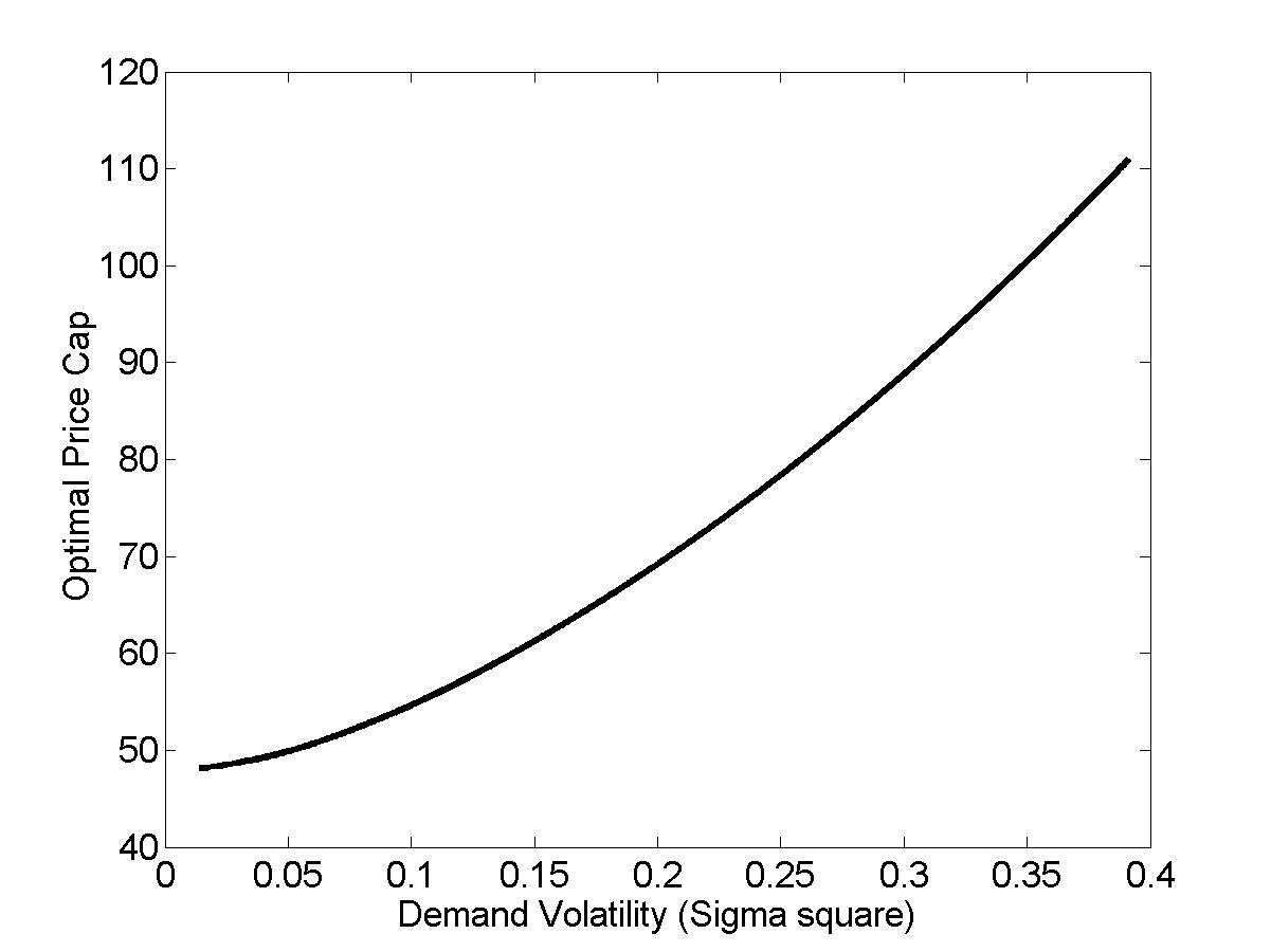
2.4 Impact of price ceiling regulation Figure 2.3: Optimal price cap vs. demand volatility C = 600, σ2 = 0.3, µ = 0.03, γ = 0.6, ρ = 0.08 Proof See Appendix 4.
This result generalizes Dobb's(2004) result which is obtained in the case of a monopoly. Figure illustrates that the bounds of the interval (P min, P ) depend on market concentration. The less competitive the industry, the lower P min and the larger P . Figure shows the impact of demand volatility on the optimal price cap P opt.
The effect of price cap regulation on investment incentives under oligopolistic competition is not monotonic with respect to the price cap due to two effects working in opposite directions: the option value effect and the strategic underin- vestment effect.
A price cap has a negative impact on the value of new capacity. It caps po- tential upside profits while leaving unchanged potential downside losses, thereby providing a disincentive to investment. In order to commit new capacity, firms require demand pressure to be high and hence the price cap to be binding for some time. Hence a tighter price cap implies that a greater current pressure of demand is necessary to trigger new investment, thereby becoming a disincentive for investment.
2.4 Impact of price ceiling regulation As explains in his model of perfect competition: If the imposed price cap is so low that at this point the return on capital is only just above the normal rate, then investors want to be assured that this state of affairs will last almost forever before they will commit irreversible capital.
Under symmetric oligopolistic (Cournot) competition without price cap, the value maximizing strategy of a firm is not to increase capacity as quickly as the perfectly competitive market in order for prices to increase. However, when there is a binding price cap the optimal strategy might change. An infinitesimal increase in capacity will not lead to a reduction in price, the price cap will still be binding, but it will lead to an increase in profits because each firm is producing and selling more. Hence a price cap provides an incentive to invest in new capacity. In other words, a price cap reduces the ability of firms to leverage their market power by keeping capacity low. Consequently, a tighter price cap should reduce the investment price trigger P and thereby induce more investment.
A price cap has therefore a dual impact on the investment price trigger of an oligopolistic industry. This explains the two regimes observed in figure Over the interval (P opt, P ∗), the positive effect of the price cap on strategic underin- vestment dominates the negative impact of the price cap on the option value of waiting, so that the investment price trigger P is an increasing function of the level of the price cap P . For a price cap lower than the competitive entry price P opt, the impact of the price cap on the option value of waiting dominates, such that the investment price trigger P is a decreasing function of the level of the price cap P .
Moreover, the implementation of a price cap lower than P min would be coun- terproductive, as it raises the investment price trigger above the oligopolistic investment price trigger without a price cap. As the price cap is lowered to zero, the investment price trigger tends towards infinity, as in the case of perfect 2.5 Sensitivity analysis and simulations Sensitivity analysis and simulations In this section we investigate the effectiveness of price cap regulation and the robustness of the price cap. We conclude the section with a comparison of long term prices and average installed capacity in the presence and in the absence of sensible price cap regulation.
Price cap effectiveness In section 4 we found that under uncertainty price cap regulation cannot force firms' investment strategies to be identical to the strategies of firms in a compet- itive industry. This was illustrated in figure Even at the optimal price cap, there will be underinvestment compared to the perfect competition and firms will earn positive rents.
In this section, we quantify how effective a price cap can be in retrieving the Definition 11 We define the price cap effectiveness coefficient  by P ∗(P ) − P ∗ where P ∗ is the investment price trigger for the unregulated industry, P investment price trigger when the regulator caps prices at P , and P ∗ is the investment price trigger of the unregulated competitive in- Maximum effectiveness is achieved when the regulator imposes the optimal price ceiling (P opt). In this special case, the effectiveness coefficient is given by ∗ = N γ − (N γ − 1)(1 − The price cap effectiveness coefficient  takes the value of one if the price cap retrieves the perfect competition investment strategy and it is zero if the price cap does not change the Cournot oligopolistic investment strategy 1An interesting extension left for further research would be to study the impact of a price 2.5 Sensitivity analysis and simulations Figure 2.4: Maximum effectiveness vs. demand volatility Price Cap Efficiency Demand Volatility Figure shows that price cap regulation is more effective for less concen- trated markets. This has a straightforward explanation closely related to the strategic underinvestment effect. In a highly concentrated market, unregulated firms have an incentive to be very slow in investing in new capacity in order for prices to increase. A price cap reduces the ability of firms to leverage their market power in order to increase prices - although not completely as firms can still play on the timing of new investments. The more competitive the market, the less market power can be leveraged by firms rendering the price cap less useful.
More interestingly, figure shows that the effectiveness of price cap regu- lation is crucially dependant upon how uncertain demand is. High demand un- certainty tends to make price cap regulation ineffective. This can be intuitively explained by the option effect. Uncertainty (measured here by demand volatil- ity) makes the option to defer investment in new capacity valuable; a company wants to be fairly sure that it will recoup the irreversible cost of investment be- cap on market efficiency, i.e. on a measure of social welfare such as the sum of firm profits andconsumer surplus. A proper evaluation of the latter would require a more detailed study ofquantity rationing and explicit modeling of consumer surplus.
2.5 Sensitivity analysis and simulations fore committing to invest. A price cap reduces the upside potential gains without affecting the potential downside losses, therefore making it necessary for a firm to wait for even higher demand before committing to invest. Therefore increased uncertainty reduces the effectiveness of price cap regulation because it amplifies the value of postponing investment.
Robustness of price cap regulation As it is evident from figure the price cap that maximises investment incentives is the global minimum of the function P . In the previous section we investigated how effective this price cap is in making the market more competitive. Another interesting issue for a regulator is the question of how robust the optimal price cap is to model parameters. This has important implications for regulators in markets where demand volatility is difficult to estimate and is subject to structural breaks or macroeconomic shocks.
Figure shows that the optimal price cap depends crucially on demand volatility. For example, if volatility is missestimated to be 10% instead of 20% the optimal price cap will be misscalculated to be 54.7 instead of 69.2. What is the magnitude of the impact of such a large (21%) underestimate of the optimal price cap on investment? In this section we concentrate on this question by defining a robustness coef- ficient and investigating the trade-off between price cap effectiveness and robust- ness. We also examine the effect of not taking into account the uncertainty in demand when setting the price cap. We find that, as a rule of thumb, it is better to overestimate demand volatility and to set a price cap that is too high rather than setting a price cap that is too low.
Trade-off between robustness and effectiveness Definition 12 We define the robustness (r) of a price cap as: where P min is the smaller solution of P (P ) = P ∗.
2.5 Sensitivity analysis and simulations Figure 2.5: Robustness vs. effectiveness Robustness Vs Effectiveness Robustness coefficient In other words, it is the lowest price cap that produces an investment price trigger equal to the price trigger of the unregulated industry. Any price cap lower than P min would be counter productive as it raises the investment price trigger. So the robustness coefficient is a measure of how much error in the estimation of the price cap it takes in order for the price cap to be counterproductive and slow down investment.
As can be seen from figure a regulator can choose to increase the robust- ness of the price cap by setting a price cap that is higher that the optimal price cap. However, this comes at a loss of effectiveness. The new price cap does not speed up investment as much as the optimal price cap. We investigate this trade Figure shows that price cap regulation is not only more effective the more concentrated the market is, but is also more robust. Furthermore, it is possible to increase the robustness of a price cap but this happens at the expense of 2.5 Sensitivity analysis and simulations effectiveness. The upper part of each graph corresponds to price caps set higher than the optimal level, while the lower part of the graph represents price caps set lower than optimal. Figure shows that setting the price cap higher is always better than setting it lower than the optimal price cap because of the effectiveness A general insight from our model is that it is better to overestimate demand volatility than it is to underestimate it. Significant underestimation has the potential to make regulatory intervention counterproductive by slowing down investment beyond the level of the unregulated oligopolistic market. In contrast, significant overestimation can only render the price cap irrelevant; it will not slow down investment.
Market evolution and the long term effect of price In this section we aim to provide some insights on the magnitude of the investment delays caused by the exercise of market power and the effect of optimal price cap regulation. We simulate several realizations of the stochastic demand and we observe the corresponding capacity expansion and price Simulation parameters The parameters for the simulation model were chosen to be representative for We do not pretend to offer a precise characterization of investment in electricity markets due to the model's stylized nature (e.g. for a more realistic, but static two period model of price caps in electricity markets). Rather, the aim of this section is to provide some insights into the order of magnitude of the quantitative impact on the delays and underinvestment identified in the previous sections.
Electricity markets are characterized by several features that make them a good test case for our model. Electricity markets exhibit high demand volatility and in many regions are not very competitive.
both these reasons, a variety of price control mechanisms related to technical 1Numerical solutions and simulations were implemented in MATLAB. The code is available from the authors upon request.
2.5 Sensitivity analysis and simulations Base case parameters Fixed investment costs Demand growth (µ < ρ) Risk free discount rate Number of firms (N > 1/γ) Initial production quantity Optimal Price cap Initial inverse demand Figure 2.6: Base case simulation parameters dispatch constraints or market power mitigation procedures are suspected to have a detrimental impact on investment incentives. This is particularly the case for peaking units which earn most of their revenues at periods of high prices (e.g.
Table summarizes the default simulation parameters. Initial capacity is normalized to one as we are interested in comparing the relative level of invest- Figure shows one path of realized prices in three cases: perfect competition, unregulated oligopoly and optimally regulated oligopoly. The investment price trigger of the regulated oligopoly is lower than the investment price trigger of unregulated oligopoly, but remains higher than the investment price trigger under perfect competition. The lower right hand side figure shows the evolution of capacity in all three cases. It shows that although the regulated oligopoly is investing more in new capacity than the unregulated oligopoly, it still does not invest as much as the competitive industry.
This section presents a Monte Carlo simulation to gain some insight into the long term effects of price cap regulation on both investment in new capacity and 2.5 Sensitivity analysis and simulations Figure 2.7: Price and capacity evolution for one demand realisation Oligopoly (N=3) without Price Cap Oligopoly (N=3) with Optimal Price Cap Investment Trigger Investment TriggerReal Price Perfect Competition Evolution of Capacity Perfect Competition Investment Trigger Oligopoly with Optimal Price Cap C = 600, σ2 = 0.3, µ = 0.03, γ = 0.6, ρ = 0.08, N = 3, X0 = 160.
average prices.
Impact of price cap on capacity installed We compute the average installed capacity after 10 years over 10,000 demand re- alizain the case of unregulated oligopoly, regulated oligopoly and perfectly competitive industry and calculate the following ratios: • QOlig represents the ratio of the average installed capacity after 10 years of an unregulated oligopoly to that of the perfectly competitive industry.
• QOPC represents the ratio of the average installed capacity after 10 years of a regulated oligopoly to that of the perfectly competitive industry.
Table shows the extent of underinvestment caused by market power for a range of values of the base-case parameters of table The results of the 1The standard errors using 10,000 were always less than 4%.
2.5 Sensitivity analysis and simulations Figure 2.8: Average installed capacity after 10 years (expressed as % of compet-itive market capacity) simulation suggest that the impact of imperfect competition on installed capacity can be quite significant. Both the unregulated as well as the unregulated firms install on average only 69% and 78% respectively of the perfectly competitive industry capacity after 10 years (assuming base-case parameters). Table shows also that variations of the investment cost, growth and volatility of demand, price elasticity and market concentration significantly impact both the extent of underinvestment and the efficiency of price cap regulation.
Impact of price cap on long term average price Similarly, we run a Monte Carlo simulation to compute the average price markup after 10 years over 10,000 demand realizations in both a non-regulated oligopolis- tic industry and a regulated oligopolistic industry with an optimal price cap as compared to the competitive price, and compute the following ratios: • POlig represents the ratio of the average price after 10 years in a non- regulated oligopolistic industry and in the perfectly competitive industry.
• POPC represents the ratio of the average price after 10 years in a regulated oligopolistic industry with an optimal price cap and in the perfectly com- petitive industry.
Table shows the mark-up over the competitive price for varying values of the base-case parameters introduced in Table 11. The average price in the non-regulated oligopolistic industry represents on average 193% of the average Figure 2.9: Average markup over competitive price after 10 years competitive price after 10 years with the base-case parameters. The average price in the regulated industry represents on average 139% of the competitive price.
Table 3 shows also that variations of the investment cost, volatility of demand, load growth, price elasticity, and market concentration significantly affect the mark-up in both the non-regulated and the regulated oligopolistic industries.
We study the effect of price cap regulation on investment in new capacity in a con- tinuous time model of a Cournot oligopolistic industry with stochastic demand.
We find that a relatively high price cap can speed up investment compared to the unregulated industry, while a stringent price cap will become a disincentive for investment.
On the practical side, we find that regulatory intervention in the form of a price cap is more effective when the market is concentrated and there is relatively little demand uncertainty. The impact of parameter estimation error in the optimal price cap is asymmetric, as underestimation can be much more damaging than overestimation. We complement this intuition using Monte Carlo simulation to confirm that a sensibly regulated market has higher capacity and lower average price compared to the unregulated market.
These results yield important practical insights for regulators, shedding light on some of the potential pitfalls of price cap regulation when there is significant demand uncertainty and investment is largely irreversible. For the utilities in- dustry, and in particular the electricity industry, our findings give some weight to the defenders of higher wholesale electricity market price caps in the US, who argue that the current price caps are too low and will lead to delayed investment in peaking units In the light of our model, regulators might be more effective in inducing invest- ment in new capacity by removing barriers to entry. Making electricity markets more competitive has for instance been the primary objective of the UK regula- tor, which first imposed price caps during the years 1994-1996 before forcing two waves of power plant divestures to the dominant companies Further work is in progress to extend our intertemporal approach under un- certainty to price cap regulation. We are in particular investigating the effect of a construction time-lag between the decision to invest and the time at which the new capacity becomes operational. Furthermore, it would be interesting to confront our model results with some empirical studies measuring the effect of regulatory interventions on investment incentives. In a recent attempt, empirically investigates the effect of zoning laws and growth control statures that attempt to limit urban sprawl by placing restrictions on the allow- able density of new housing developments. He finds that the imposition of controls is not as effective as anticipated because it destroys the option value of waiting.
His empirical findings confirm the theoretical predictions of our theoretical model regarding price regulation.
We want to show that in the absence of variable costs profit maximizing firms produce at full capacity provided that N γ > 1.
Proof The profit of firm i is given by equation The marginal profit result- ing from a marginal increase in quantity produced is given by ∂π = XQ−1/γ − 1/γXQ−1−1 Given that q = Q , If we N γ > 1, the marginal profit is always positive ( ∂π > 0), therefore firms will always produce at full capacity.
The characteristic equation of the differential equation is: 1 σ2β(β − 1) + µβ − ρ = 0.
The equation has roots The general solution of the differential equation takes the following form mi(P (Q), Q−i, q) = H0P β1 + H1P β2 + A0P + B0 where H0,H1,A and B are constants A0P + B0 is the particular integral of the differential equation, with A = Nγ−1 Since β2 < 0, H1 = 0 otherwise the term H1P β2 would tend to infinity as P approached zero.
Using the two boundary conditions and yields after some algebra the analytical expression of the investment price trigger P ∗ given in equation and H0 is given by N γ(µ − ρ)β N γ(µ − ρ) β1 (N γ − 1)(1 − β1) Solving the stochastic optimal control problem of equation using requires to distinguish two different regimes depending on demand: 1. Non-binding price cap (P ≤ P ) mi(P, Q−i, qi) = H1P β1 + 2. Binding price cap (P ≥ P ) mi(P, Q−i, qi) = H2P β1 + H3P β2 + with β1 > 1 and β2 < 0 given by equations The marginal value satisfies the two free boundary conditions: Value matching condition at the investment trigger P m(P , Q−i, qi) = C Smooth pasting condition at the investment trigger P (P , Q−i, qi) = 0 Continuity of value and fist derivative at the price cap P give two additional boundary conditions: , Q−i, qi) = mi(P where the notation P refer respectively to the limit of the function evaluated below and above the price cap P The system of four equations and with four un- knowns (H1, H2, H3, P ) defines the symmetric Nash Cournot equilibrium invest- ment strategies of a firm when prices are capped at P . An analytical expression of these four equations is given below by equations and This system is non-linear but can be solved analytically.
From equation and and from equations and where we introduce α = to simplify notation.
Equating and to eliminate H3 gives (β1−1) − β1 We can use the expression of β1 and β2 to simplify this equation. Since β1 and β2 are the two roots of the characteristic equation of they satisfy the following two relations: β1 + β2 = 1 − which can be manipulated to give [(β2 − 1)(β1 − 1)].
Using the expression above, together with α = the equation of the optimal investment price trigger P becomes In this appendix we prove that there exists an interval (P min, P max) over which the introduction of a price cap lowers the investment price trigger as compared to the oligopolistic industry investment trigger without price cap (i.e. P ≤ P ∗).
We will also show that the upper limit Pmax is equal to the investment trigger without a price cap P ∗.
Define ∆ = P − P ∗ the difference between the industry investment price trigger with and without price cap (P ). To demonstrate proposition it is sufficient to prove that ∆ ≤ 0 over the interval [P min, P max].
− (β2 − 1)P )P ∆ ≤ 0 is equivalent to − (β2 − 1)P )P − P ∗β2 ≥ 0 where we have used the fact that β2 < 0. This can be rewritten as It can be shown graphically that this equation has two solutions. Furthermore, it can be shown by direct substitution that the larger of the two solutions is the unrestricted price trigger (P = P ∗). This is intuitively what one should expect since a price cap higher than the unrestricted investment price trigger is irrelevant.
It is not possible to find the other solution (P min) analytically.
− (β2 − 1)P )P Differentiating this expression with respect to the price cap P and setting the derivative to zero we obtain the optimal price cap: The second order condition at P opt can be shown to be ∂2P > 0 which implies that P opt is indeed a minimum.
Amstrong, Mark, David Sappington. 2005. Recent developments in the theory of regu- lation. Mark Amstrong, Robert Porter, eds., Handbook of Industrial Organisation, vol. 3. Amsterdam: North-Holland, 295–384. Baldursson, F. 1998. Irreversible investment under uncertainty in oligopoly. Journal of Economic Dynamics and Control 22 627–644. Beesley, M., S. Littlechild. 1989. Regulation of privatized monopolies in the United Kingdom. RAND Journal of Economics 20(3) 454–472. Biglaiser, G., M. Riordan. 2000. Dynamics of price regulation. RAND Journal of Economics 31 744–767. Cowan, S. 2002. Price-cap regulation. Swedish Economic policy Review 9 167–188. Cunningham, Christopher R. 2006. Growth controls, real options and land develop- ment. Forthcoming . Dixit, A. 1991. Irreversible investment with price ceilings. Journal of Political economy Dixit, A., R. Pindyck. 1994. Investment under uncertainty. Princeton University Press.
Dobbs, I. 2004. Intertemporal price cap regulation under uncertainty. Economic Journal Earle, R., K. Schmedders, T. Tatur. 2006. On price caps under uncertainty. Working Ghemawat, P., B. Nalebuff. 1990. Exit. RAND journal of economics 16 184–194. Gilbert, R.J., R.G. Harris. 1984. Competition with lumpy investment. RAND journal of economics 15(2) 197–212. Grenadier, S. 2002. Option exercise games: an application to the equilibrium investment strategies of firms. The Review of Financial Studies 15(3) 691–721. Grobman, J., J. Carey. 2001. Price caps and investment: long-run effects in the electric generation industry. Energy Policy 29 545–552. Hagerman, J. 1990. Regulation by price adjustment. RAND Journal of Economics 21 Huisman, K.J.M., Peter M. Kort, Grzegorz Pawlina, Jacco Thijssen. 2003. Strategic investment under uncertainty: Merging real options with game theory. CentER Discussion Paper . Joskow, P., J. Tirole. Forthcoming. Reliability and competitive electricity markets.
RAND Journal of Economics . Laffont, J.-J., J. Tirole. 1993. A theory of incentives in procurement and regulation.
Laffont, J.-J., J. Tirole. 2001. Competition in Telecommunications. MIT Press. Lambrecht, Bart. 2001. The impact of debt financing on entry and exit in a duopoly.
Review of Financial Studies 14(3) 765–804. Leahy, J. 1993.
Investment in competitive equilibrium: The optimality of myopic behaviour. The Quarterly Journal of Economics 108(4) 1105–1133. Littlechild, S. 1983. Regulation of british telecomunications' profitability. London: Department of Industry . McDonald, R., D. Siegel. 1986. The value of waiting to invest. The Quarterly Journal of Economics 101(4) 707–727. Metcalf, G., K. Hassett. 1995. Investment under alternative return assumptions: com- paring random walks and mean reversion. National Bureau of Economic Research Technical Working Paper 175. Murto, P., E. Nasakkala, J. Keppo. 2004. Timing of investments in oligopoly under uncertainty: A framework for numerical analysis. European Journal of Operational Research 157 486–500. Newbery, D. 2005. Electricity liberalisation in britain and the evolution of market design. Energy Journal . Phillips, Owen R., Charles F. Mason. 1996. Market regulation and multimarket rivalry.
RAND Journal of Economics 27(3) 596–617. Pint, E. 1992. Price-cap versus rate-of-return regulation in a stochastic-cost model.
RAND Journal of Economics 23(4) 564–578. Stoft, S. 2002. Power Systems Economics - Designing Markets for Electricity. IEEE Press, John Wiley & Sons. Trigeorgis, L. 1996. Real Options: Managerial Flexibility and Strategy in Resource Allocation. MIT Press, Cambridge, MA. Price ceilings with time-to-build In this Chapter we extend the study presented in Chapter 2 on the effect of price cap regulation on investment in new capacity to allow for a time lag between the commitment to build new capacity and this capacity becoming operational.
First we solve the problem for a monopolist and then generalize to a symmetric We find that for stringent price cap regulation, time-to-build amplifies the disincentive for new investment already present in models without time-to-build.
For higher price caps we find that time-to-build creates a bifurcation: It results in three locally stationary investment strategies. We characterize the solutions and provide an intuitive explanation for these results. Rather surprisingly this paper shows that sensible price cap regulation is more effective with increasing time-to-build, something rather encouraging from a regulatory point of view.
Keywords: Real options, price cap regulation, time-to-build, bifurcation, monopoly, JEL code: C73, D92, L51, L94.
Investment in new capacity is typically a lengthy process. The international en- ergy agency reports that in the power generation industry, the time lag between deciding to build a new power plant and the commencement of production, spans at best between three years for a gas turbine and six years for a nuclear plant This includes the time required to obtain regulatory and local approval, the actual construction period, and the final testing and commissioning stage. Similarly, finds a two to three year time lag in real estate development investments. reports a ten year lag in pharmaceu- tical R&D projects, while construction of an underground mine requires more than 5 years to complete Empirical studies have demonstrated that construction time lag is an impor- tant factor to be considered in the investment strategy of a firm, in particular when profitability is uncertain. examine a capacity mix model under demand uncertainty that explicitly accounts for differences in technology lead times. Subsequently, they show that lead time is a key design pa- rameter that needs to be considered by investors alongside capital and operating Several theoretical real options models have been developed to investigate this important aspect of investment under uncertainty both in isolation, for ex- ample and as well as in competitive equilibrium, for example and Despite the practical importance of construction time lags in investment deci- sions, their effect on price cap regulation is a relatively unexplored area. Although the effect of price cap regulation under uncertainty has recently been investigated in both a one-time period moas well as in a more dynamic framewthese studies assume instantaneous capacity expansions. This study extends the work presented in Chapter 2 on the effect of regulatory intervention in the form of a price cap on investment in new capacity to include this important feature which occurs in almost all industries.
1For example show that under uncertainty a price cap that is close to long run costs will fail to reduce prices.
2For example studies the effect of price cap regulation on the investment de- cisions taken by a monopolist in a real options model, while Chapter 2 extends the investigationin similar settings to an oligopoly.
The general framework of the model is the standard real options approach to investment under uncertainty: a firm facing stochastic demand decides whether to invest in completely irreversible capacity that requires θ years to build. Solving the problem for the optimal investment strategy (both timing of investment and quantity) in the presence of time lags is generally speaking difficult because the path dependency (capacity that is being built but is not yet operational) makes the size of the state space very large. However, using a result from we are able to show that the investment strategy with time-to-build is identical to the investment strategy of an artificial market in which all com- mitted capacity (both completed and capacity that is being built) is considered completed and operational. This result reduces the state variable space from infinitely many to just two variables: the level of committed capacity and the demand. This allows us to solve the problem using standard real options tech- In order to explain our findings it is necessary to consider what the effect of a time lag is in the simplest setting. The presence of a time lag in a model with deterministic demand is usually a disincentive to investment. Since a firm would be required to pay for the investment up-front and only receive a positive cash flow at the end of construction, it would require a higher return on its investment to be compensated for the time value of money.
Similarly to deterministic models, real options models with stochastic demand show that a price cap is a disincentive to investment. and show that a construction time lag slows down investment: it will increase the level of demand pressure necessary to trigger investment in new capacitNamely, Grenadier finds that the optimal investment strategy in the presence of a time lag is to invest whenever the discounted expected price at the end of construction is equal to the price trigger without time lags. That is, firms wait until they are expecting to recover their irreversible investment plus an extra premium for the time value of money.
1The level of demand that would trigger investment in new capacity is often referred to as demand investment trigger (see Since in our models the priceis an one-to-one function of the demand, the level of demand that triggers investment in newcapacity has a unique price associated with it. We refer to this price as the investment pricetrigger.
In the presence of price cap regulation, we find that for relatively low price caps (close to the deterministic competitive market entry price) the demand pres- sure that would trigger investment in new capacity is higher than the equivalent without time-to-build. However, overall the price trigger is a decreasing function of the price cap for any time-to-build. This happens because of the option value of delaying investment: since the price cap limits the upside potential of the in- vestment, but not the downside risk, a firm would rather postpone investment until the demand pressure was quite higThe time lag simply amplifies the value of the option because of the time value effect.
In the absence of time-to-build, as the price ceiling is raised, the investment trigger becomes an increasing function of the price ceiling due to it preventing strategic underinvestment as explained in Chapter 2. This happens until the price cap reaches the unregulated industry entry price above which price cap regulation becomes irrelevant. In the presence of time lags the investment price trigger with time-to-build exhibits a bifurcation. There are now three locally stationary investment strategies, two maxima and one minimum.
this difference occurs because of a new effect. In the absence of time lags a firm would invest as soon as the marginal increase in value from a new unit of capacity is equal to the construction costs. In the presence of time lags, the optimality condition for investment in new capacity is to increase capacity when the marginal value of the firm is equal to the construction cost, plus the cost of lost revenue while the new unit is being built. Effectively, time lags increase the economic cost of investment in new capacity. This new effective cost depends on price and is capped by the price cap. Although overall the price cap destroys value because it limits the upside potential of future revenues (option effect), it is possible that it provides an incentive for investment because it reduces the effective costs of construction. For very low price caps the destruction of value is too great for a price cap to provide an extra incentive for investment. Yet as the price cap increases this disincentive becomes smaller. This provides the 1For a more detailed description of this effect see Chapter 2 or pages 300-1.
firm with two possible strategiethe first is the traditional recoupment strategy: since costs are higher, wait longer before investment. The second strategy is the cost preemption strategy; since the effective investment costs are increasing with price, invest heavily in order to reduce the price and therefore reduce the overall costs. Both the cost preemption and the recoupment strategies are local maxima.
To determine the global maximum, the problem for the value of the firm must be solved and use this to characterize the solutions. We find that for low price caps the recoupment strategy is the global optimum, while for higher price caps the preemptive strategy performs better.
We show that our results with time-to-build are compatible with existing models. In the limit of the time-to-build going to zero the results of this study recover to the results presented in Chapter 2. On the other hand, as the price caps tends to infinity, our results recover Grenadier's results of unregulated investment with time-to-build Finally, we believe that our results are interesting from a real options point of view. The combination of time-to-build and price cap regulation creates a multiplicity of solutions. This is a phenomenon that, to the best of our knowledge, has not been observed before in similar models.
Finally, we extend our study of intertemporal price cap regulation with time- to-build from a monopolistic industry to a symmetric Cournot oligopoly. The complication here is that the investment decisions will depend not only on the stochastic demand, as was the case for the monopolist, but also on the capacity and capacity evolution of all agents in the market. The strategic interactions make the problem more difficult to solve as we are solving a system of simultaneous optimization problems. We use similar methodology to Chapter 2 to solve this problem. As in models without price caps, for example and we find that there is more investment in new capacity in more concentrated markets. Price cap regulation has the potential of speeding up investment even further, but since in less concentrated markets there is less market power to start with, there is less scope for regulatory intervention.
1What we find is in fact three locally stationary strategies one of which is a minimum. This is a consequence of the fact the new solutions always appear in minima/maxima pairs. Sincethis is a local minimum it is not of particular interest.
We also present sensitivity analysis and a simulation results. Our aim is to examine the robustness of regulatory intervention and quantify the increase in investment when a sensible price cap is in place. We find that due to the multiplicity of solutions, the optimal price cap level is very sensitive to market parameters (such as volatility and time-to-build). Nevertheless, it is still possible to have a sensible price cap that speeds up investment in new capacity.
Generally speaking, our findings are encouraging from a regulatory point of view. This is because relatively high price caps, that would only ever be bind- ing during construction and only if firms do not invest early enough, can have a beneficial effect in speeding up investment in the presence of market power.
Furthermore, these price caps are not often binding, reducing the problem of raa which a regulator would otherwise have to face.
The rest of the paper is organized as follows. Section 2 introduces the model of investment under uncertainty for a monopolist, formulates the profit maximiza- tion problem as a problem of stochastic optimal control and demonstrates how to reduce the state space to two variables. In section 3 the problem investment trigger of the firm is determined, whilst in section 4 we solve for the value of the firm. Our results are extended to a symmetric oligopoly in section 5. We study the optimal price cap and investigate its robustness in section 6 along with sim- ulation results. Final conclusions and suggestions for further research are then presented in section 7.
Consider a monopolist facing stochastic demand. The inverse demand function is given by the following expression: P (t) = X(t)C(t)− 1γ 1Rationing occurs when the price cap is binding because there is more demand than supply in the market. The exact rationing process is beyond the scope of this paper.
where C(t) is the quantity produced and γ is the demand elasticitX(t) is the stochastic component of demand which we assume to follow a geometric Brownian dX = X(t)µdt + X(t)σdz where µ is the drift of the demand process, σ is the instantaneous standard devia- tion and dz is a Wiener process. For our problem to have non-trivial solutions we assume µ < ρ where ρ is the (continuously compounded) time value of money Furthermore, we assume that the the market is elastic enough (γ > 1) so that the marginal profit of the firm is increases in X(t). This assumption guarantees that provided that there are no variable costs the firm will always produce at full capacitFor the rest of the paper we will assume that the quantity produced is equal to the operational capacity available in the market.
As long as no new capacity becomes operational, the produced quantity re- mains constant and the market clearing price given by the inverse demand func- tion of equation follows the stochastic process: dP = P (t)µdt + P (t)σdz The profit of the monopolist will depend on how many units the firm is selling and the price it can charge: π(X(t), C(t)) = min(P (t), P )C(t) = min(X(t)C(t) γ , P C(t)) where P is given by equation and P is the price cap imposed by the regulator.
That is, when the price is lower than a predetermined level P chosen by the regulator then consumers must pay the price given by equation to purchase a unit of the monopolist's production. On the other hand, when the price is higher than P consumers must only pay P to purchase one unit of the production and 1For a justification of why a demand specification in the form of equation might be a reasonable approximation, as well as a critique, see 2Under complete markets hypothesis ρ is the risk free interest rate. If markets are not complete then ρ is a subjective required rate of return.
3If we relax this assumption the model becomes a two-stage problem: the monopolist would first have to decide how much to produce up to her capacity constraint and then if she wantsto invest in more capacity. A real options model that examines this is excess demand is rationed by the regulator in an efficient way. In this case, the price P (t) given by equation is not the real price but instead it is a hypothetical market clearing Investment in new capacity costs K per unit and is completely irreversible.
We also assume that investment in new capacity is infinity divisible. Construction in new capacity takes θ years to complete, where θ is the time-lag between the time t at which the firm takes the decision to increase capacity, and t + θ the time at which this capacity becomes operational.
Let Ct denote the operational capacity at time t, Bt the capacity that is being built (but not yet completed) at time t, qt = Bt +Ct the total capacity (both oper- ational and in the pipeline) at time t and Λt = {t ∈ (t−θ, t) s.t. lim Bk > lim Bk} the set of times when new capacity was added to the pipeline but has not yet become operational. Note that qt−θ = Ct since all capacity in the pipeline at time t − θ will be operational at time t.
Let Ωt = {Xt, Ct, Bt, Λt} denote the information available at time t and ΩA = {Xt, qt, 0, ∅} denote the information of an artificial economy in which all capacityin the pipeline is treated as completed.
The optimization problem of a firm maximizing profits at time t = 0 is to choose the path of investment q(t) that maximizes the expected present value of future cash flows: e−ρtπ(X(t), q(t − θ))dt − Ke−ρtdq(t) Ω0] The first term represents the discounted expected operating revenue from com- pleted capacity from time zero onwards, while the second term represents invest- ment costs in new capacity. This is a problem of stochastic optimal control, where the control parameter is the capacity installed.
This is a difficult problem to solve because the state variable space Ωt can be very large. It includes all points in the past θ years at which commencement of construction of new capacity occurred (Λt). Fortunately, following 1The market clearing price, when higher than the price cap, is also referred to as shadow price, for example, see p.297.
as used by the state space of the optimization problem can be transformed to the two variable space ΩA. The result is summarized in the following proposition: J (Ω0) = J(ΩA)+ e−ρtπ(X(t), q(t − θ))dt Ω0] − E[ e−ρtπ(X(t), q(t − θ))dt ΩA] Proof See Appendix 1.
The optimization of the first term is not path dependent and there are only two state variables, the committed capacity (both completed and being built) and the demand. There is no optimization over the path dependent second term.
The above result has a simple intuitive explanation. The investment strategy of a firm with several units at different stages of construction is identical to the investment strategy of a firm that has all of its capacity completed and operational. This is because the firm has to make a decision that will only become effective after θ years. So what matters when making this decision is not current capacity but capacity θ years down the line. However θ years later all capacity in the pipelines will be completed. In fact, θ years later a firm with capacity in the pipelines will be identical to a firm that currently has all of its capacity completed. Therefore, their investment strategies have to be the same. That is not to say that the values of the two firms are the same. It is the timing and size of future expansions decisions that are the same. The difference in value of the two firms is given by the second and third term of equation The third term is the expected discounted revenue from capacity that is being built at time t = 0 as if it was operational immediately (without time-to-build). Since this capacity is not operational it is subtracted from the value of the firm. The second term is the expected discounted revenue of capacity that was already being constructed at time t = 0 as it becomes operational in the interval t ∈ [0, θ]. Since this is an 1Although was published before Grenadier refers to their 1992 working paper for this result.
3.3 Investment price trigger extra revenue that the firm receives it has a positive sign. This result simplifies the problem and allows us to use Ito's lemma to solve this stochastic optimal control problem, which we will do in the next section.
Looking at this problem with a real options lens, the monopolist has a series of call options on capacity.
When existing capacity (both completed and in the pipelines) is q(t), the monopolist receives an instantaneous dividend equal to π(X(t), q(t − θ)). Yes she also has the option to invest in new capacity. The strike price of this option is Kdq. The optimization problem is how high must the pressure of demand be for the monopolist to exercise this option. NPV analysis would suggest that the monopolist should exercise this option as soon as the discounted expected future revenue is equal to the investment cost. However, this ignores the irreversibility of investment. By investing now in an infinitesimal capacity increase, the monopolist is giving up the right to invest in the future.
Classic options analysis dictates that the monopolist should wait until this option is deep in the money before investing.
However the situation here is a bit more complicated than simple option pric- ing for two reasons. The first is that the price is endogenous. So when the mo- nopolist invests in new capacity she increases the supply available to the market, therefore decreasing the price. Thus new capacity (when it becomes operational) reduces the revenue stream from all existing capacity. So when the monopolist increases capacity she should take into account the negative impact of a capacity increase to the rest of her revenues. The second difference is that when the firm exercises the option to expand capacity, immediately another option becomes available, the option to further expand capacity. Therefore, we can view this as an infinite number of compound options and will use Ito's lemma to price them simultaneously in the next section.
Investment price trigger For the rest of the paper we will consider a firm which at time t = 0 has no capacity being built (B(0) = 0), making the operational capacity equal to the 3.3 Investment price trigger total capacity C(0) = q(0Let the value of such a firm, pursuing the optimal investment strategy, be V (X, q) = J (ΩA). Consider the infinitesimal interval between t and t + dt over which no investment takes place. The value of the firm at time t will have two components. The first is the cash flow from production during the time interval dt and the second is the expected continuation value beyond that short time interval suitably discoun V (X, q) = π(X, q) + E[V (X(t + dt), q)e−ρdt] Using Ito's lemma and expanding the exponential term, ignoring terms of higher order than O(dt), when there is no expansion of capacity, the value of the firm must satisfy the following differential equation: 1 σ2X2VXX + µXVX − ρV + π(X, q) = 0 For what follows it will be very helpful to define the marginal value of the firm as m = ∂ V (X, q). Note that since there is no new capacity being committed to between t and t + dt this is a change of variables we are allowed to perform. The partial marginal value will follow: σ2X2mXX + µXmX − ρm + π(X, q) = 0.
Furthermore, it will be useful to change variables from X(t) to P (t). Note that this change of variable is permitted as long as no capacity is added to the system.
Using equation ∂ = q−1/γ ∂ , and changing variables results in: σ2P 2mP P + µP mP − ρm + π(P (X, q), q) = 0 1There is no loss of generality with this assumption. The investment policy of a firm with capacity in the pipelines is identical to that of the firm with the same capacity but all of itcompleted, as shown in proposition Their values differ by the last two terms of equationover which no optimization takes place.
2Since the demand (and hence the price) is stochastic, the continuation value is also stochas- tic. Therefore, we will need to use an expectation for the continuation value.
3.3 Investment price trigger The general solution of equation is standard in the real options literature, e.g. and takes a different form if the price cap is binding.
If the price cap is not binding (P < P ), the general solution of the equation m(P, q) = H1P β1 + H0P β2 + While if the price cap is binding (P ≥ P ), the solution of the equation is of m(P, q) = H2P β1 + H3P β2 + where β1 and β1 are the roots of the characteristic equation of the differential 1 σ2β(β − 1) + µβ − ρ = 0 The two roots are: with β1 > 1 and β2 < 0.
In order to solve this ordinary differential equation completely we need to determine the constants H0, H1, H2, H3 using the relevant boundary conditions of the problem. One condition is that when demand is sufficiently high, new investment is triggered. As part of the solution we expect to find an optimal expansion policy in the form of a price trigWhen this price is reached, it triggers investment in new capacity. If there were no time lags, the new capacity would immediately reduce the price through equation The price trigger would therefore act as a reflecting boundary for the market clearing price. For further discussion on the investment trigger in the absence time lags see Chapter 2 or Chapter 9.
When a price cap above the investment price trigger is introduced in the absence of time lags it will simply be irrelevant. It will never be reached because the investment price trigger is a reflecting boundary for the price process. So the 1The stochastic process that we have chosen for the demand given by equation satisfies the conditions necessary for the investment strategy to be a trigger strategy as discussed in Appendix B, Ch4.
3.3 Investment price trigger price cap must be lower than the price trigger in order to have any effect at all.
In such a case, the price level that would trigger new ivestment is not the real price consumers are paying. It is rather the hypothetical market clearing price (or shadow price in the terminology of that would have prevailed if there were no price caps.
In the presence of time lags the situation is more complicated. Naturally, there is still a price level that triggers new investment. When it is reached the firm will commit to new capacity which will take θ years to be constructed.
During construction, the price can (and most likely if µ > 0 will) increase. The investment trigger is no longer a reflecting boundary and the actual price can go above the price trigger. Of course as soon as the new capacity becomes operational the price will drop, but that does not happen for θ years. Now if a price cap is introduced it can clearly have an effect even if it is above the price trigger.
This happens because such a relatively high price cap can be binding during To solve the problem we need to distinguish two cases according to the rela- tionship of the investment price trigger and the price cap.
Case 1: Price cap is higher that the investment price trigger. In this such a case the price cap can only ever be binding while new capacity is in the pipeline but has not yet become operational. The solution is of the form of equation subject to the boundary conditions: BC1: Since P = 0 is an absorbing barrier for the price process, the marginal value of the investment at any level of committed capacity should be zero.
BC2: When the price trigger P ∗ is reached, the firm will invest in an infinites- imal amount of new capacity dq. If this is done optimally, the value of the firm with the extra unit of capacity dq in the pipeline minus the construction cost must be equal to the value of the firm without the new capacity. This is usually referred to as the value matching condition. Using the fact that V (X∗, q) = J (X∗, q, 0, Ø) 3.3 Investment price trigger where X∗ = P ∗q1/γ at the point of entry the value matching condition is V (X∗, q) = J (X∗, q, dq, Ø) − Kdq Using the transformation of equation we can write the equation above as: V (X∗, q) =V (X∗, q + dq) + E[ e−ρtπ(X, q)dt X(0) = X∗] e−ρtπ(X, q + dq)dt X(0) = X∗] − Kdq We can express the above equation in the derivative form and change variables from X(t) to P (X, q): Let Z(P ∗) be the integral Z(P ∗) = E[R θ e−ρt ∂π(P,q) dt P (0) = P ∗] which we eval- uate in Appendix 2.
BC3: Also, at the entry point, the value must satisfy the smooth pasting Since these conditions are on the marginal value of the firm µ(P, q) we will need another condition in order to determine the value of the firm V (X, q) uniquely.
BC4: As the supply in the market goes to infinity there is zero probability of new investment and there is zero probability that a nonzero price cap will ever be binding. Therefore, the value of the firm will be equal to the expected present value of operating with capacity q forever. This is summarized by the condition: lim V (P (q), q) = These conditions define the optimal exercise policy and the value the firm uniquely for the case of high price caps.
1See Appendix C, Chapter 4 for an intuitive demonstration of the smooth pasting condition or for a derivation.
3.3 Investment price trigger Case 2: Price cap is lower than the investment price trigger. In this case, investment can only take place while the price cap is binding, provided the demand pressure expressed by the hypothetical market clearing price P (t) of equation is high enough. Nevertheless, it is possible for the price cap to be binding and no investment to be taking place. Let m1 be the general solution given by equation and m2 the solution given by equation The general solution will have to satisfy the same boundary conditions as the previous case: m2(P ∗, q) = Z(P ∗) + K lim V (P (q), q) = With the additional condition that the two regimes must meet continuously and smoothly at the price cap (see m1(P , q) = m2(P , q) It is useful to understand the intuition behind the investment trigger bound- ary conditions given by equations and The Gaussian integral Z that appears in these expressions can be interpreted as the discounted expected revenue of a marginal unit of capacity for the next θ years. Since the marginal unit of capacity is being built during these θ years, Z can be thought of as the expected lost revenue due to the fact that capacity is not operational immedi- ately, but only after θ years. In the absence of time-to-build (lim firm would invest at the price that made the change in value of the firm with extra capacity equal to the cost of construction. In the presence of time-to-build 3.3 Investment price trigger however, the firm will invest once the change in value of the firm is equal to the construction cost plus the cost of lost revenues due to the time lag. So time lag increases the effective construction cost of new capacity. As we shall see later this extra cost plays an important role in the optimal strategy of the firm. But first, let us summarize the optimal investment policy in the following proposition: Proposition 14 The investment price trigger with time-to-build P ∗ is given by equation provided that it exceeds the price cap P . Otherwise, it is given by P ∗β2 = λP 2−1(M (P ∗) + K − α(ρ − µ)(M (P ∗) + K) θ Φ(v(P, t) − u(t)) P e−(ρ−µ)t + (1 − Φ(v(P, t)))P e−ρt]dt, Φ is the cumulative normal distribution, v(P, t) = log(P /P )−(µ−σ2/2)t Proof Straight forward from solving the free boundary problem specified above.
The integral Z(P ) is evaluated in Appendix 2.
These equations cannot be solved analytically because of the integral Z(P ) in- volving Gaussian integrals, but they can be studied numerically. We will do this at the end of this section. However, first it is interesting to investigate the asymp- totic behavior of equations and in two cases: as time-to-build goes to zero and as the price cap goes to infinity.
3.3 Investment price trigger Asymptotic behavior of investment price trigger Time lag tends to zero Provided the price cap is not very high (P /P ∗ < 1), as the time lag θ goes to zero, the Gaussian integral limθ→0 Z(P ) = 0 and limθ→0 M = 0. Equation becomes identical to the expression derived in for the investment price trigger of a regulated monopoly without time lags.
On the other hand, if the price cap is set relatively high (P /P ∗ > 1), as the time lag θ goes to zero and limθ→0 M = 0 and equation becomes identical to the investment price trigger derived in For an unregulated economy without time-to-build: We retrieve the result that high price caps (higher than the competitive entry investment trigger) are irrelevant in the absence of time-to-build.
Price cap tends to infinity For finite time-to-build θ, as P → ∞ intuition suggests that the price cap should become irrelevant. Indeed, lim Z(P ) = R θ P e−(ρ−µ)tdt = P 1−e−(ρ−µ)θ which is equivalent to the formula given in for the investment trigger of a monopoly without price ca Investigation of investment price trigger A graphical investigation of the price trigger P with time-to-build θ = 0.5 and θ = 3 years appears in figures and respectively. What we observe from figures and is that for low price caps the effect of time-to-build is to delay investment in new capacity until the pressure of demand is higher than the case without time-to-build. The longer the time lag, the more a monopolist would delay investment. This is easy to understand. Since the company is making an upfront investment of K, which will only start generating income θ years in 1There are a few differences between Grenadier(2000) and this formulation. Here we are working with the marginal value m(P, Q) instead of the total value V (P, Q). Also the statevariable is not the demand X but the shadow price P = XQ−1/γ . Furthermore, Grenadier wassolving the optimization problem of a central planner trying to maximize consumer welfare.
His formulation can be straightforwardly applied to a monopolist maximizing profits.
3.3 Investment price trigger the future, the demand hurdle that would trigger new investment needs to be higher. The firm needs to be quite sure that there is a good chance that there will be a high price when the unit become operational (or at least the price cap will be binding for a long time). Only then will it be able to recoup its, substantial investment costs. Accounting for this difference the picture resembles the picture of investment without time-to-build. The investment price trigger is a locally convex function of the price cap due to the two competing effects described in detail in Chapter 2. Namely, the option value effect and the strategic Yet more interestingly, as the price cap increases further we observe three locally stationary investment triggers emerging. Why does this bifurcation oc- cur? From the boundary condition the monopolist will invest only if the marginal value of the firm, with respect to an increase in capacity, is equal to the cost of building the capacity (K) plus the (expected) cost of lost revenue due to the time required to build the capacity. The firm treats the lost revenue as an extra cost, which is necessary to pay in order to invest in new capacity. Although the real cost of investment in new capacity is independent of time-to-build, the effective cost of investment is higher the longer the time-to-build because of the cost of lost revenues during construction.
Since capacity is effectively more expensive with time-to-build, the firm delays investment even more in the presence of time-to-build. This strategy is attempt- ing to recoup the effective costs of new investment. This explains why the highest locally optimal trigger (blue colour) occurs.
In the presence of a price cap, this extra cost is bounded from above by P (1 − e−ρθ) ' P θ as the most the company loses (per unit time) from the new capacity not being operational is P and the total duration of construction is θ.
Therefore, for a low price cap the extra cost is relatively modest. As the price cap increases this cost can become substantial, thus forcing the firm to wait for even higher prices before investment, as it tries to ensure that it will recoup the cost of new capacity. However the firm realizes that it has another possible strategy. It can try to reduce the effective cost of new capacity by decreasing the price. After all, if the price is low the cost of lost revenue is also low. The firm preemptively invests in new capacity in order to drive the price down and with it 3.3 Investment price trigger Investment price trigger vs Price cap (Theta = 0.5 years) Investment Price Trigger (IPT) Figure 3.1: Investment price trigger vs. price cap, θ = 0.5 years K = 600, σ2 = 0.3, µ = 0.03, γ = 1.2, ρ = 0.08, Time-to-Build = 0.5 years Investment price trigger vs Price cap (Theta = 3 years) Investment Price Trigger (IPT) Figure 3.2: Investment price trigger vs price cap, θ = 3 years K = 600, σ2 = 0.3, µ = 0.03, γ = 1.2, ρ = 0.08, Time-to-Build = 3 year 3.3 Investment price trigger the effective cost of new investment. This is a cost preemption strategy. As the price cap is further increased and exceeds the investment trigger (so it can only ever be binding during construction) the monopolist still invests more quickly than she would have done if there was no time lag. This is because the price cap reduces the effective cost of investment. In the limit where the price cap goes to infinity, the price cap no longer reduces the effective costs since it will never be binding. Consequently the investment price trigger asymptotically approaches the unregulated investment price trigger from below. The cost preemption strategy is the green line solution in figures and What is interesting is that there is a region where both the cost recouping and the cost preemption strategies are locally optimal. This is the region over which the bifurcation occurs. From what we have done so far it is not possible to determine which strategy (delay investment in order to recoup increasing effective costs or speed up investment in order to decrease effective investment costs) is the global maximum. We will investigate this question in the next section. However, before we go there let us try to understand what the third locally stationary solution (red line) represents.
Whenever a one-dimensional (non degenerate) nonlinear system exhibit a multiplicity of stationary points, new stationary points must appear in pairs. Furthermore, for each pair of new solutions, one must be a local minimum and the other a local maximum, and maxima and minima alternate each other (see for example This explains the third solution (red line on figures and It is a local minimum strategy that lies between the cost recoupment and cost preemption strategies. This strategy is of no important significance, however it must exist because between two local maxima there must be a minimum.
In order to verify the intuitive characterization of the investment strategies presented above and also to determine which strategy is the global maximum, we need to solve for the value of the firm. We proceed to do this in the next section where we also discuss which of the two investment strategies is the global 3.4 Value of the firm Value of the firm The value of a firm following the investment price trigger that was derived in Proposition is summarized by the following proposition.
Proposition 15 The value of a firm with operational capacity q facing price P at time t = 0 and no capacity in the pipeline is: If the price cap is not binding (P < P ) while if the price cap is binding (P ≥ P ) then [−K − Z(P ∗) − P ∗ZP (P ∗)]( 1 − 1 γ − β1 where P ∗,Z(P ),λ and α are given in Proposition Proof Straight forward from solving equations and using the invest- ment strategy of Proposition and the boundary condition These equations have an intuitive explanation. The last term of equations and is the present value of all future cash flows from assets already 3.4 Value of the firm in place. The first term represents the present value of all increases in capacity.
It includes the cost of building new capacity (both actual and effective costs), the lost value due to the reduction of price from the introduction of new capacity and the extra revenue from having a new unit of capacity in operation. For relatively low price caps the situation is more complicated. The third term of equation is the present value of all future cash flows from capacity that is already operational provided the price cap remains bounding for ever. The first term of equation is similar to the first term of equation The second term of equation that appears for the first time, is the present value of all lost future cash flows that are forfeited due to the price cap not being binding.
Note that for the value of the firm to satisfy the boundary condition it is necessary to assume that the market demand elasticity γ < β1As points out, if that is not the case the industry cannot exist; the value of the firm in such an industry is always negative.
The introduction of the price cap reduces the value of the firm. As the time lag increases the value of the firm decreases as illustrated in figure This is because the time lag increases the effective cost of construction due to the time value effect. Yet what is interesting to observe is the value in the area of the bifurcation. Clearly the cost preemption strategy (blue line) is the globally optimal solution for higher price caps than the recoupment strategy. The third stationary solution, being a minimum is always less (or equthan the other two strategies.
The fact that there is a cross over from the cost preemption to the recoupment strategy as the level of regulatory intervention decreases has important implica- tions for the optimal regulation of this market. Before we examine this in section we investigate the effect of price cap regulation in an oligopolistic industry.
1We have already restricted the demand elasticity γ to be more than 1 in order for the monopolist to produce at full capacity. The assumption 1 < γ < β1 might seem restrictive butthere is a wide range of µ, σ, ρ that allows this. Furthermore, as we shall see in the next section,oligopoly changes this condition to the less strict 1 < γ < β 1 where n is the number of firms active in the industry.
2The equality occurs at the point where the bifurcation first appears and at the point where it first disappears.
3.4 Value of the firm Firm Value vs Price cap Unregulated firm value Figure 3.3: Value of the firm vs. price cap 3.5 Equilibrium investment of a symmetric oligopoly Equilibrium investment of a symmetric oligopoly In this section we extend our model from a monopoly to an oligopolistic industry with time-to-build. Oligopolies are interesting from a practical perspective since a number of industries, for example electricity markets, are not dominated by a single agent but by a relatively small number of agents. As a result oligopolies exhibit imperfect competition. The study of an oligopoly is more difficult because of the dynamic interactions between agents. The strategy space is much larger because each firm will base its decision to invest in new capacity not only on the stochastic demand, but also on the actions of all other firms in the industry.
An appropriate solution concept for such a game is the Nash equilibrium: no agent benefits from changing his strategy. In mathematical terms we are solving n simultaneous stochastic optimal control problems by finding a fixed point in the strategy space of all agents. Fortunately, we can use a simplification of this challenging problem, as first suggested by essentially the Nash equilibrium solution of a competitive market, under certain conditions, coincides with a single agent maximization problem. This result is also used by and to demonstrate that the Nash equilibrium option exercise policy of a symmetric oligopoly is equivalent to the solution of a single agent maximization problem.
We can readily use this result to extend our study of price cap regulation from monopoly to oligopoly of n profit maximizing firms. Let q(t) = (q1(t), q2(t), ., qn(t)) be the vector of committed capacities of all firms in the market (both operational and in construction) at time t, and Q(t) = qj be the aggregate capacity available in the market. We define similarly c(t) to be the vector of operational capacities and C(t) the aggregate operational capacity, b(t) to be the vector of capacity under construction and B(t) the aggregate capacity under construction and Λt the sets of times that new capacity was initiated in the previous θ years:{Λt}i = {t ∈ (t − θ, t) s.t. lim B(k)i > lim B(k)i}}. The information available at time t = 0 is summarized with Ω0 = {X(t), c(t), b(t), Λt}.
3.5 Equilibrium investment of a symmetric oligopoly The inverse demand function of such an industry will be given by P (t) = X(t)C(t)−1/γ and the profit of firm i at time t will be πi(X(t), C(t), ci(t)) = min{X(t)(C(t))−1/γci(t), P ci(t)} The optimization problem for each agent in the industry is: e−ρtπi(X(t), qi(t − θ), Qi(t))dt − Ke−ρtdqi(t) Ω0] To solve the Nash equilibrium problem we have to solve the system of n stochastic optimal control problems simultaneously. Fortunately, we do not need to do this as we can use the result proven in that the Nash equilibrium investment strategy of a symmetric economy is equivalent to the investment policy of a myopic firm that ignores the possibility of entry by compe- tition. This result allows us to solve the problem as a single agent optimization problem. In Chapter 2 we also used this result to find the equilibrium investment strategy of an oligopoly without time-to-build. Here we extend these results to the case of price cap regulation with time-to-build.
For a symmetric economy qi(t) = qj(t) = q(t) = Q(t)/n ∀i, j ∀t ∈ [0, ∞). This transformation reduces the state space considerably. Following the same steps as for the monopoly, we obtain the following differential equation for the marginal value mi of the myopic firm (that ignores competitive entry): + µP mi − ρmi + The last term of the left hand side is the marginal profit of the myopic firm: πi(P (X, Q), q) = min{P We can follow the same steps as in the previous section to derive the optimal investment trigger of the myopic firm which coincides with the optimal investment 3.6 Optimal price cap trigger of the oligopoly. The following proposition summarizes the investment trigger for a symmetric oligopoly.
Proposition 16 The investment price trigger with time-to-build P ∗ is given by equation provided that it exceeds the price cap P . Otherwise, it is given by P ∗β2 = λP 2−1(M (P ∗) + K − α(ρ − µ)(M (P ∗) + K) θ Φ(v(P, t) − u(t)) P e−(ρ−µ)t + (1 − Φ(v(P, t)))P e−ρt]dt, Φ is the cumulative normal distribution, v(P, t) = log(P /P )−(µ−σ2/2)t Proof Straight forward from solving equation The effect of competition is to change the constant α which in turn has the effect of reducing the investment price trigger. In order to avoid preemption firms will not wait for as long as they would have liked to in the absence of competition. This erodes the value of waiting. The more concentrated the market, the bigger the dilution of the value of the option to wait. This is illustrated in figure A market with three agents is quicker to invest and the investment trigger is uniformly lower for all price caps. However, the qualitative picture remains unaltered. There is still a region of multiple solutions which have the same intuitive explanation as the monopolistic case.
Optimal price cap In the absence of time-to-build the investment price trigger is a convex function of the price cap. In such a case it is easy to find the optimal price cap, the price 3.6 Optimal price cap Investment price trigger vs Price cap Investmet Price Trigger Figure 3.4: Investment price trigger at different levels of competition K = 600, σ2 = 0.175, µ = 0.03, γ = 1.2, ρ = 0.08, time-to-build = 1.5 years cap that minimizes the investment price trigger is the global optimum. It is also robust against small changes of parameters.
In the presence of time-to-build the price trigger is no longer a convex function of the price cap, making the task of finding an optimal price cap more difficult. We define the optimal price cap as the price cap that results in the lowest investment price trigger. For example, the monopolist presented in figure has a locally optimal strategy to invest in new capacity when the shadow price is 148 provided that the price cap is also set at 148. However, as is obvious from figure the globally optimal strategy for the firm when the price cap is 148 is to invest when the shadow price is equal to almost 495! As can be seen in figure the truly optimal price cap (optimal in the global sense) is much higher around 283. Such a price cap would produce an investment price trigger of 235. This is remarkably lower than the investment trigger of the unregulated economy (879), but not as low as the competitive market (146).
The problem with the optimal price cap is that it is not robust with respect to small variations in model parameters. If ,for example, the regulator estimates the parameters even slightly wrongly (or the firm perceives them a bit differently), 3.6 Optimal price cap Globally Optimal Investment Price Trigger vs Price Cap Optimal Investment Price Trigger Figure 3.5: Globally optimal investment price trigger vs. price cap K = 600, σ2 = 0.175, µ = 0.02, γ = 1.2, ρ = 0.08, time-to-build = 3 years, n = 1 this would lead to suboptimal regulation. The smallest of increases in demand volatility would increase the optimal investment price trigger by more than 200% (from 235 to 578).
This happens because, as is evident from figure the globally optimal price cap is the smallest price cap that makes the cost preemption strategy the globally optimal investment trigger. This is the smallest price cap that would trigger investment without it being binding. When some model parameters change, such as a small increase in variance, the preemption strategy is no longer the global optimum, the recoupment strategy is. The monopolist will no longer invest just before the price cap is binding, instead she will wait until the price cap is binding and the shadow price is high enough to ensure that there is a good chance that she will recoup the irreversible cost of investment.
Nevertheless, sensible price cap regulation is still possible. Fairly high price caps, that would only be binding during construction, can have a very beneficial effect. They would generally provide an incentive to speed up investment and could be robust against variations in model parameters, albeit that robustness 3.6 Optimal price cap Globally Optimal Investment Price Trigger Vs Price Cap, n=3 Optima Investment Price Trigger Figure 3.6: Globally optimal investment price trigger vs. price cap K = 600, σ2 = 0.175, µ = 0.02, γ = 1.2, ρ = 0.08, time-to-build = 3 years, n = 3 comes at a loss of efficiency. We study the trade-off between the effect of a price cap and its robustness in the next section.
As we move from a monopoly to a higher market concentration there is less scope for regulatory intervention. As can be seen in figure an oligopoly of 3 firms has an unregulated investment price trigger of 203. This is more than 4 times less than the unregulated price trigger of the monopolist and 15% less than the best achievable through price cap regulation. The intuition behind this is straight forward; the more concentrated the market, the closer it gets to the competitive outcome. Since there is less market power to start with the price cap becomes less efficient in mitigating market power. This is shown in figure Trade off between price cap effectiveness and ro- In this section we investigate in more detail the trade-off between the effectiveness and robustness of the price cap. On the one hand, the regulator would like to 3.6 Optimal price cap choose the price cap level that reduces the investment trigger as far as possible.
On the other hand, the regulator would also like to have a price cap level that is robust to small variations in model parameters, for example demand volatility.
As we have seen in the previous section the globally optimal price cap level is not robust. Therefore, the regulator is presented with a dilemma, increase the price cap in order to obtain robustness at the expense of efficiency or cap aggressively and increase efficiency at the expense of robustness.
In order to study the trade-off between robustness and effectiveness we need to quantify them. We define the robustness coefficient as the maximum (%) allowable error in the price cap that maintains the preemption strategy as the globally optimal strategy.
where P go is the globally optimal price cap.
To quantify efficiency, we need a measure of how close price cap regulation brings the economy to the competitive outcome. Define d be the distance be- tween the trigger of a regulated economy at P with the competitive investment . Similarly, let D be the distance between the trigger of the unregu- lated economy to the competitive investment trigger D. We define the efficiency coefficient as 1 − d .
For example, if the regulator sets the price cap at the true global optimum price cap level P go, the robustness coefficient will be zero. This is because any price cap smaller than P go will change the global optimal to the cost recoupment trigger but it has effectiveness e(P go), which is the best a regulator can hope for. In contrast, in the limit where the price cap goes to infinity (no price cap regulation) the robustness coefficient is 1 while the effectiveness coefficient is zero.
This denotes that any error is not going to have an effect on the price trigger, but at the same time the price cap does not speed up investment compared to 3.6 Optimal price cap Robustness vs Efficiency Robustness of Price Cap regulation 0.2 Efficiency of Price Cap regulation Figure 3.7: The trade-off between price cap effectiveness vs robustness K = 600, σ2 = 0.175, µ = 0.02, γ = 1.2, ρ = 0.08, time-to-build = 3 year, n = 1 the unregulated market. Figure shows the trade-off between effectiveness and robustness with the data of figure Simulation of regulated market with time-to-build Simulation results for a monopolistic industry are presented in figure We confirm that the capacity installed with sensible price cap regulation is always greater than capacity installed in a free market. Furthermore, we confirm that a time lag of three years induces further investment in capacity which becomes operational three years later. So the committed capacity (that is both operational capacity and capacity in the pipelines) is always greater in the presence of time lags when the regulator imposes a sensible price cap. That is not to say that the economy is better off with a three year time-to-build instead of 0. Although the capacity that the firm would commit to is larger when the time-to-build is three years than if it is instantaneous, it still takes three years for this capacity to become operational. So during these three years the economy with the zero Table 3.1: Simulation parameters Base case parameters Fixed investment costs Demand growth (µ < ρ) Risk free discount rate Number of firms (n > 1/γ) Initial production quantity Optimal price cap (θ=3 years) Optimal price cap (θ=0 years) Construction time lag time lag is better off.
We have studied price cap regulation under uncertainty in the presence of time-to- build. The most interesting aspect of the model is the appearance of a bifurcation.
There are a range of price cap levels where there are two meaningful strategies for the firm. The reason behind this is that the effective cost of construction depends on price and is an increasing function of the price cap. The first strategy is to wait for high prices before investing in order to recoup the higher costs associated with the time lag. The second is to actively reduce the cost of investment by investing earlier in new capacity therefore decreasing the price.
There are five factors that contribute to the appearance of multiple solutions: • Stochastic demand. This could be a more general process than the geomet- ric Browning motion used in this model.
• Endogenous price that is a decreasing function of supply. It is essential that there is a trade off between increasing capacity and reducing price.
• Irreversible investment.
Regulated monopolist (theta=3y) Regulated Monopolist (theta=0y) Optimal Price cap Investment Trigger Investment Trigger Optimal Price cap Unregulated Monopolist (theta=0y) Installed Capacity Investment Trigger Regulated (theta=3y) Regulated (theta=0y) Unregulated (theta=0y) Figure 3.8: simulation results K = 600, σ2 = 0.175, µ = 0.02, γ = 1.2, ρ = 0.08, n = 1 • Exogenous constraints on the price process. Such as a price cap or indeed any other form of constraint.
• Time lag between committing to new capacity and the capacity becoming It would be interesting to investigate whether or not other problems of invest- ment under uncertainty exhibit such nonlinear dynamics with multiple solutions when a time lag is introduced. For example, inventory control models under un- certainty. When the inventory cost is an increasing function of the number of units stored, there are constraints on the number of items ordered and it takes time for orders to be delivered then non-linear dynamics might be exhibited.
Our model provides some useful insights for regulators. It proves to be sensible to implement a price cap when firms exhibit market power, provided that it is rather high. Such a price cap can only be binding while new construction is taking place and only if firms do not invest early enough. Furthermore, it will encourage investment in new capacity, thus reducing long-term prices without having a negative impact on the security of supply. Sensible regulation in the presence of different technologies with different lead times is an interesting challenge that we leave as further research. However, we note that price regulation in the form of a price cap might discriminate against some technologies, and not necessarily the ones with the longest lead times.
Appendix 1: proof of proposition The optimization problem of equation can be re-written as: π(P (t), q(t − θ))e−ρtdt Ω0] π(X(t), q(t − θ))e−ρtdt Ω0] − We have broken down the revenue into two terms. The first is the revenue in the interval (0, θ) from capacity committed in the past θ years. The second term is revenue from capacity already existing at time zero plus any potential new capacity. Note that decisions to invest in new capacity at time t = 0 do not affect the first term due to the time lag θ: Only investment decisions taken in the θ years before t = 0 affect the first term.
Another interesting observation is that although the expectation depends on the investment path over the last θ years (Λ0), the optimization depends only on the capacity Q0 committed at time t = 0. In other words we can the optimization term is independent of when new capacity went into the pipeline. Therefore equation we can change the information set in equation from Ω0 to ΩA: π(X(t), q(t − θ))e−ρtdt Ω0] π(X(t), q(t − θ))e−ρtdt ΩA] − Finally we change the limit of integration of the optimization term from θ to 0 and we subtract the appropriate integral at the end: π(X(t), q(t − θ))e−ρtdt ΩA] − π(X(t), q(t − θ))e−ρtdt Ω0] − E[ π(X(t), q(t − θ))e−ρtdt ΩA] (3.41) which can be re-written as: J (Ω0) = J(ΩA)+ π(X(t), q(t − θ))e−ρtdt Ω0] − E[ π(X(t), q(t − θ))e−ρtdt ΩA] Appendix 2: calculating Z(P) We will use the properties of geometric Brownian motion to estimate the expected present value of future marginal cash flows from time t = 0 to t = θ when the current price is P and the price is capped at P .
e−ρtdt P (0) = P ] The firm's cash flow is given by: π(q, X) = min Xq−1/γq, P q e−ρtdt P (0) = P ] = ∂ E[min(P (t), P )e−ρt P (0) = P ]dt = R θ E[P(t)e−ρt P ≤ P , P (0) = P ]dt + R θ E[P e−ρtI where Ia<b is the indicator function: I = 1 if a < b and zero otherwise.
Following the shadow price at time t ≤ θ is P (t) and given current price P0 is lognormally distribute log P (t) ∼ N (log P0 + (µ − Using the following two properties of the lognormal distribution: 1. The expected value of x is E(x) = eg+s2/2.
2. When x is truncated from above at x0 then the expected value of x is given by E(x x ≤ x0) = Φ(u−s) eg+s2/2, where Φ denotes the cumulative distribution function of the standard normal and u = 1 (log x θ Φ(v(P, t) − u(t)) P e−(ρ−µ)t + (1 − Φ(v(P, t)))P e−ρt]dt where v(P, t) = log(P /P )−(µ−σ2/2)t , u(t) = σ t.
Appendix 3: proof of propositions and In this Appendix we estimate the value of the firm (summarized by Proposition by solving the free boundary problem outlined in Section 3.3. As part of the solution we determine the investment price trigger that maximizes profits (which is summarized in Proposition We start with the second part of the propositions (where the investment price trigger is lower than the price cap P ∗ < P ) which is simpler to analyze. In this case the marginal value of the firm is given by equation m(P, q) = H1P β1 + H0P β2 + where β1 > 1 and β2 < 0. The three boundary condition are given by the 1At time t = θ the shadow price will experience a downwards jump because the new capacity whose construction commenced at time t = 0 will become operational. However for 0 ≤ t < θover which the integral Z(P ) is calculated, the shadow price is lognormally distributed.
m(P ∗, q) = Z(P ∗) + K lim V (P (q), q) = Since β2 < 0 the first condition implies that H0 = 0 otherwise the value of the firm would go to infinity at the origin.
Substituting equation in conditions BC2 and BC3 we get: Solving these two equations we get equation which is the second part of the Proposition α(ρ − µ)(M (P ∗) + K) In order to solve for the marginal value of the firm we need to determine H1.
Using equations and we get [Z(P ∗) + K + P ∗ Thus we have determined the marginal value of the firm and we need to integrate it with respect to quantity in order to determine the total value of the firm. The integration gives: where c is the constant of integration. Using BC4 we can show that c = 0.
Substituting H1 in the expression above we can get the expression for the value of the firm given in the second part of proposition Turning our attention to the case where the investment price trigger is below the price cap (P ∗ ≥ P ), the expression for the marginal value of the firm will depend on whether the price cap is binding or not. If the price cap is not binding, the marginal value of the firm is given by equation m1(P, q) = H1P β1 + H0P β2 + When the price cap is binding the marginal value of the firm is given by equation m2(P, q) = H2P β1 + H3P β2 + where β1 > 1 and β2 < 0. The six boundary condition are given by the following m2(P ∗, q) = Z(P ∗) + K lim V (P (q), q) = m1(P , q) = m2(P , q) The first condition implies that H0=0. BC2 can be written as Multiplying the last equation with and subtracting it from the previous BC5 can be written as while BC6 can be written as These last two equations can be solved in terms of H3 to give: We can solve equations and to get the investment price trigger of equation which is the first part of Proposition P ∗β2 = λP 2−1(M (P ∗) + K − In order to determine the value of the firm we will need expressions for H1 and H2. From equation we get an expression for H2 in terms of H3 and from equation we get an expression for H1 in terms of H3 and H2: Similarly to the case where the price cap is larger than the investment price trigger, the value of the firm is determined by integrating the marginal value of the firm given by equations and and using BC4 to estimate the constant of integration. The final value is: If the price cap is not binding (P < P ) while if the price cap is binding (P ≥ P ) then which concludes the proof of Proposition Aguerrevere, Felipe L. 2003. Equilibrium investment strategies and output price be- havior: A real-options approach. Review of Financial Studies 16(4) 1239–1272.
Baldursson, F. 1998. Irreversible investment under uncertainty in oligopoly. Journal of Economic Dynamics and Control 22 627–644. Bar-Ilan, A., W.C. Strange. 1996. Investment lags. American Economic Review 86 Bar-Ilan, A., A. Sulem, A. Zanello. 2002. Time to build and capacity choice. Journal of Economic Dynamics & Control 26 69–98. Dixit, A., R. Pindyck. 1994. Investment under uncertainty. Princeton University Press.
Dobbs, I. 2004. Intertemporal price cap regulation under uncertainty. Economic Journal Earle, R., K. Schmedders, T. Tatur. 2006. On price caps under uncertainty. Working Gardner, D., J. Rogers. 1999. Planning electric power systems under demand uncer- tainty with different technology lead times. Management Science 45(10) 1289– Grenadier, S. 1995.
The persistence of real estate cycles.
Journal of Real Estate Economics 8 95–119. Grenadier, S. 2000. Project flexibility, Agency, and Competition, chap. Equilibrium with Time-to-build: A Real-options Approach. Oxford University Press. Grenadier, S. 2002. Option exercise games: an application to the equilibrium investment strategies of firms. The Review of Financial Studies 15(3) 691–721. IEA. 2003. Power generation investment in electricity markets. IEA, Paris. Jongen, H.Th, P. Jonker, F. Twilt. 2000. Nonlinear Optimization in Finite Dimensions.
Kluwer Academic Publishers, Dordrecht. Leahy, J. 1993.
Investment in competitive equilibrium: The optimality of myopic behaviour. The Quarterly Journal of Economics 108(4) 1105–1133. Majd, S., R. Pindyck. 1987. Time to build, option value and investment decisions.
Journal of Financial Economics 18(1) 7–28. Merton, R.C. 1973. Theory of rational option pricing. Bell Journal of Economics and Management Science 4 141–181. Murto, P., E. Nasakkala, J. Keppo. 2004. Timing of investments in oligopoly under uncertainty: A framework for numerical analysis. European Journal of Operational Research 157 486–500. Schwartz, Eduardo S. 2004. Patents and R&D as real options. Economic Notes 33(1) Real options in partnerships We study partnership contracts under uncertainty but with clauses that admit downstream flexibility. The focus is on the effects of flexibility on the synergy set, which constitutes the core of the contract. In a partnership context the value of flexibility is captured by the partners who own the right to exercise their options. On one side there are cooperative options, which are exercised jointly and in the interest of maximizing the total contract value. On the other side there are non-cooperative options, which are exercised unilaterally, or by coalitions, in the interest of the option holders' payoffs. We provide a modelling framework that captures the effects of optionality on partnership synergies. We study these effects under a complete markets assumption, based on standard contingent claims analysis, as well as under heterogenous risk-aversion, using a dynamic programming model. The model shows the effect of several strategies on the synergy set and the bargaining position of the partners. It also shows that non-cooperative options, if agreed prior to negotiation, are powerful bargaining tools but that they can also destroy the partners' incentive to participate in the contract. Finally, the model illustrates how risk sharing provides larger synergies for partners with heterogeneous risk attitudes.
Partnerships are a driving force of the modern economy. Joint ventures between car manufacturers, alliances between airlines, co-development contracts between pharmaceutical and biotech companies, production sharing contracts between oil majors and national oil companies, are but a few industries where partnerships are significant drivers of value.
Partnerships aim to create synergies by combining core competencies of the partners to form a distinctive offering that neither partner could provide alone.
Synergies are traditionally thought of in terms of improved efficiency, e.g. through economies of scale or scope. In an uncertain world, however, there are at least two further important sources of synergies: risk sharing and flexibility. Risk sharing is particularly interesting if partners have different risk attitudes, e.g. as with a pharmaceutical major and a small biotech company, enabling win-win situations by trading-off risks. Additional flexibility in a partnership can have significant value by allowing partners to cut downside risk or amplify upside potential as the uncertain future unfolds. In this paper we will explore such stochastic synergies.
The framework for most partnerships is provided by a legal contract. Two key questions in contract negotiations are: How should the contract be structured to generate significant total value at an acceptable level of risk? How should this total value and the associated risks be shared amongst the partners? These chal- lenges are exacerbated when long-term partnerships are negotiated in volatile commercial environments. Mitigating clauses tend to be included in contracts to avoid lock-in and enable partners to react, either jointly or unilaterally and without the need to breach the contract, when uncertainties unfold. The con- tract then becomes a dynamic frame. What are the implications of contingency clauses for the contract value as a whole? How do contingency clauses change the bargaining positions of the partners? These are the core questions that we address in this paper.
In our practical experience value effects of contingency clauses are often un- derestimated or even completely discarded. The reply of a senior manager to our question about the rationale for his suggested royalty rate is representative in this regard: ‘We are contributing 50% of the R&D expenditure. It seems only fair to set the royalties so that we receive 50% of the projected value if the R&D is successful'. However, his argument neglected the fact that the decision to launch the successful product was the partner's and that the manager's company would lose all royalty payment if the partner decided, for whatever reason, not to launch the new product. Flexibility can have significant value for its owner and can take away significant value from the other partners. Yet only if this value-effect is understood and taken into account in contract design and sharing negotiations can we hope to create robust partnerships that do not go sour when companies exercise flexibilities in ways that their partners had not foreseen.
The academic discussion of the fair distribution of benefits from cooperation goes back to the seminal work of and which led to the advent of bargaining theory and cooperative game theory. This literature is largely concerned with the allocation of value but not of risk. The models are mainly deterministic and combinatorial. A first strand of this literature which is relevant to our work, is concerned with cooperative game theory in the presence of stochastic payoffs, see for example We build in particular on the work of Suijs and co-workers, using the concept of a deterministic equivalent of a stochastic cooperative game, which turns out to be very useful in our analysis. A second relevant body of work focuses on efficient risk sharing and the formation of syndicates, see e.g.
for example and We integrate these two strands of literature with elements of the real options literature to study the effect of optionality in partnership contracts, an issue which, to our best knowledge, has not been thoroughly investigated to date.
Two concepts play a crucial role in the study of the value effects of uncer- tainty: diversification and optionality. Diversification is essentially a passive risk management tool and presumes no direct influence on the management of indi- vidual projects. It is therefore particularly appealing to investors. Optionality on the other hand, emphasizes the importance of pro-active risk and opportunity management and is therefore particularly appealing to managers. A right without obligation to a potential future action creates value in an uncertain environment.
The concept of optionality and its valuation in the context of financial derivatives, originated in the seminal work of and has attracted considerable academic attention and made a significant practical impact. Indeed, the concepts and approaches of financial engineering have moved beyond the design and valuation of financial instruments into the realm of capital budgeting and project valuation.
was amongst the first to advocate that significant optionality, such as growth opportunities, ought to be included in the valuation of a project or company and that the appropriate use of the work of Black, Scholes and Mer- ton might make this possible. Myers saw this as an opportunity to bridge the gap between strategy and finance and coined the term real options for this line of thinking. Shortly afterwards, illustrated how such real options could be valued with a Black-Scholes approach. These semi- nal papers, together with the monograph by spurred a significant amount of academic work over the past two decades and led to the establishment of real options as a distinct area in finance with increasing up- take in the strategy literature, see for example However the advent of real options analysis in the strategy literature has not been without controversy. We refer the interested reader to and the response to their An emerging body of literature is concerned with the relationship between optionality and competition, see for example Little work has been done to date to understand the effect of real options on the synergies created by a partnership and the consequences for fair splits of risk and return. Our aim in this paper is to fill this gap by presenting a framework that allows the investigation of contract design issues with a real options flavor. To this end, we combine concepts from cooperative game theory and real options theory - a combination that has not received the attention in the academic community that, we believe, it deserves. Our main emphasis is on the impact of options on the core of a cooperative game. The core of a contract conceptualizes a notion of a negotiation synergy set. It contains those payoff allocations for which no partner, or sub-coalition, can improve upon by going alone.
4.2 Options contracts: cooperative vs. non-cooperative options The paper is structured as follows. We begin by discussing a simple model of a cooperative real options game. In section we determine its core under three sets of assumptions, a) the existence of a complete market, b) risk neutral agents, and c) risk averse agents. In section we develop the model and insights using a more general multi-agent, continuous-time framework. Section concludes with managerial implications. In order to reach a broad readership we have structured the paper in such a way that the key intuition, illustrated by the simpler model of section can be grasped without a detailed understanding of section Options contracts: cooperative vs. non-cooperative An options contract is a contract with significant future flexibility. Options are rights but not obligations to future actions. In a partnership this raises the question of who has the right to the action? There are two types of options in partnerships depending on who has this exercise such an option.
A contract clause may specify that the decision to exercise an option is taken jointly. We call such flexibilities cooperative options and assume they will be exercised in the interest of maximizing the total value of the contract. A typical example is a decision to jointly market a product after a successful R&D effort.
Flexibility may also be owned by a single partner, or a sub-group of partners, who have the right to exercise it and will, we assume, do so in the interest of their own payoff, rather than the sum of payoffs resulting from the contract. We call such flexibilities non-cooperative options. A generic non-cooperative option on a contract is the option to breach the contract if circumstances do not unfold as anticipated, accepting possible litigation costs as the price of exercise.
The notion of a cooperative option emphasizes the collaborative nature of partnerships, whilst non-cooperative options acknowledge the transient nature of contracts and regard them as part of competitive strategies of firms who will ultimately act in their own interest. Non-cooperative options can be tacit, such as the option to breach the contract, or explicitly acknowledged in a partnership contract. For example, a clause in a co-development contract between a biotech 4.3 The core of an options contract: an illustrative model and a pharmaceutical company may allow the biotech company to opt out of fur- ther co-development and receive agreed milestone and royalty payments instead.
Formally, a non-cooperative option in a partnership can be thought of as a coop- erative game followed by a non-cooperative game. The cooperative game, i.e. the contract negotiation, sets a framework for later non-cooperative behavior, which then has to be taken into account in the negotiation.
Our main focus in this paper is the effect of flexibility, cooperative or non- cooperative, on the synergies created by the partnership. To this end we employ the notion of the core of a cooperative game, which is the set of all allocations of payoffs to the partners that will make all partners better off than without the contract. Following we illustrate option effects in the context of a very simple one-time period model with simple flip-of-the-coin uncertainty.
The model extends to more complex lattice-based and continuous-time models.
A continuous-time version is developed in Section The core of an options contract: an illustra- Assume a biotech company has a drug under development which has successfully passed all clinical trials and is now awaiting final approval by the regulator. The company estimates the present value of cash flows from the drug to be CB for a launch investment of IB < CB. The biotech company has limited production capabilities and its sales and distribution network is rather inefficient compared to pharma majors. The company is therefore negotiating a co-marketing con- tract with a large pharmaceutical company. The cash flow projection for the co-marketed product is CB+P and the launch investment will be IB+P . How should the value (CB+P − IB+P ) of the contract be shared in a fair way? The core of the deterministic game The core of this cooperative game is the set of payoff allocations that make both partners better off than if they were to go it alone. Using φB and φP to denote the 4.3 The core of an options contract: an illustrative model share of the contract value CB+P − IB+P for the biotech and pharmaceutical com- panies, respectively, and neglecting costs of capital considerations for simplicity, the core is defined by φB ≥ CB − IB = CB+P − IB+P .
In other words, the biotech's payoff share φB is in the core if CB − IB ≤ φB ≤ CB+P − IB+P , with the residual payoff φP = CB+P − IB+P − φB being allocated to the pharma- ceutical company.
Uncertain payoffs To introduce uncertainty we assume that a competitor is developing a drug that will treat the same medical condition. If the competitor is successful in developing this drug, the revenue potential of the biotech's drug will be reduced. We assume that p is the probability of failure for the competing drug. In the upside scenario of the failure of the competitor's drug, the cash flow projection if the biotech company goes alone is assumed to be uBCB, with uB > 1; in the downside scenario of competitor success, this cash flow is projected to be dBCB, with dB < 1. In the partnership the present values of the cash flows are projected as uB+P CB+P in the upside and dB+P CB+P in the downside scenario.
In section we will determine the core of this game under the assumption of complete markets. In section we replace the assumption of complete markets with risk neutral agents and we see that many of the results for complete markets carry forward. Finally, we investigate the real options cooperative game under the assumption of risk aversion in section 4.3 The core of an options contract: an illustrative model We will first examine the stochastic cooperative game under a complete markets assumption. Complete markets imply the existence of a portfolio of traded assets which replicates contract payoffs. Trading in these assets allows the partnership to hedge all risks as partners can individually short sell the replicating portfolio corresponding to their allocation of the contract payoff and thereby offset their payoffs in each state of the market. Hence the only valuation for the investment opportunity that is consistent with the absence of arbitrage opportunities is the present value of the replicating portfolio.
The risk preferences of agents are irrelevant in this situation (for details see To illustrate this effect, assume there is an asset which closely tracks the success or failure of the competing R&D project. In the case of success the price of the tracking asset will increase from P to Pu, and if the competing project fails it will decrease to Pd.
If an asset has payoffs (Xu, Xd) in the two states of the market then this payoff can be replicated with a portfolio of the tracking asset and the risk free asset, which we assume to have return r = 1 for simplicity. This replication is done by solving ψBPd + θB = Xu, ψBPu + θB = Xd, where ψ is the number of bought shares in the tracking asset and θ is the amount invested in the risk free asset.
Simple algebra shows that the value x of this replicating portfolio has the form x = ψBP + θB = qxu + (1 − q)xd, where q is given by Because 0 ≤ q ≤ 1 it is often interpreted as a probability, although its correct economic interpretation is in terms of forward prices, see The reference to q as a probability is convenient because allows the interpretation of the no-arbitrage value as an expectation under this measure. The measure q is typically referred to as the risk-neutral measure or equivalent martingale measure in the finance literature.
4.3 The core of an options contract: an illustrative model The contract without options Equation allows us to calculate the no-arbitrage value xB = quBCB + (1 − q)dBCB − IB of the contract for the biotech alone and the no-arbitrage value xB+P = quB+P CB+P + (1 − q)dB+P CB+P − IB+P for the partnership. Since under the complete markets assumption both agents would agree on these values (or allow for arbitrage opportunities), the game is reduced to a deterministic cooperative game. The value share φB of the biotech is in the core if xB ≤ φB ≤ xB+P with the residual φP = xB+P − φB going to the pharma company. The core is similar to the cooperative game without uncertainty, with the difference that the deterministic payoffs are now replaced by the no-arbitrage value of the stochastic payoffs. Effectively, trading in complete markets reduces the stochastic game to a deterministic game.
It is important at this point to make a distinction between payoff sharing and value sharing. Payoff allocations, which we will denote by (ΦB(ω), ΦP (ω)), are functions that allocate the ultimate payoffs, here uBCB+P − IB+P or dBCB+P − IB+P to the biotech and the pharma in each state of the world ω ∈ {u, d}. In each such state, the sum of the partners' payoff allocations equals the total payoff for the partnership. In contrast, the value shares (φB, φP ) are the private values which the partners assign to their payoff allocations. In our complete markets setting the payoff shares are related to the value shares by φi = qΦi(u) + (1 − q)Φi(d), i ∈ {B, P }.
Since each firm can hedge all risks through trading, the agents are indifferent between two payoff sharing rules that have the same risk-neutral value φi. In the complete markets case, the relationship φB + φP = xB+P holds.
4.3 The core of an options contract: an illustrative model A cooperative option We will now introduce a cooperative option. Suppose the companies can wait with the launch investment until they know the result of the trials for the competing drug and therefore the cash flow scenario. For simplicity we assume that there is a deterministic cost involved in waiting. Such costs may involve actual costs, such as labour costs, as well as opportunity costs, such as cost of lost sales or finite patent life etc. The waiting cost is kB for the biotech alone and kB+P for the partnership.
The biotech alone, as well as the partnership, have two possible project designs to choose from. The first is to pay kB or kB+P respectively and postpone the decision to launch until uncertainty is resolved. This will provide the option to abandon the project if the competition is successful. The alternative is not to pay the costs and as a result they will not have the option.
The method developed in the previous section can be used to price the project with the option to wait. If the biotech goes alone the no-arbitrage value B CB − IB )+ + (1 − q)(dB CB − IB )+ − kB , while the value for the partnership becomes B+P CB+P − IB+P )+ + (1 − q)(dB+P CB+P − IB+P )+ − kB+P , were q is the risk-neutral probability given by equation If the biotech alone or the partnership decides not to wait the values are given by and Knowing the values of the design alternatives the agents choose the optimal design. If xO > x B the Biotech would prefer to pay the costs involved with waiting and set up the option. If that is the case, the company would exercise the option in the states of the world where iBCB − IB > 0, i ∈ {u, d}. Similarly for the partnership. Again, the stochastic game is reduced to a deterministic game as in the previous section, with the additional complication that the agents need to also choose the optimal design and the optimal exercise policies for their 1We are using z+ as a shorthand for max{z, 0}.
4.3 The core of an options contract: an illustrative model options. The agents will choose the design with the highest risk-neutral value.
Since this is the only value that is consistent with no-arbitrage assumption, there will not be any disagreement over the value of the different designs or the optimal exercise policy. We shall see that this is not the case in the absence of markets and in the presence of risk-aversion.
The condition for the biotech's value φB to be in the core is now where x∗ is the value of the optimal design for the biotech subject to optimal x∗ = max{xB, xO}.
is similarly defined for the partnership.
A non-cooperative option To illustrate the effect of non-cooperative options let us assume that, in addition to the setting so far, the contract gives the biotech company unilateral flexibility to opt out of the co-marketing of the drug before committing to the launch cost, whilst the pharma company is locked in the contract. Suppose the biotech would receive a fixed amount Z, deducted from the contract value, if it exercised the opt-out option. The pharma will receive the residual contract value. We treat Z as an exogenous parameter and we investigate its effect on the synergy set of the The first question is how, if at all, the existence of this option changes the total value of the contract? Suppose the agents have agreed a payoff sharing rule (ΦB(ω), ΦP (ω)) if the drug is launched jointly. If the upside scenario occurs then the payoff to the biotech will be max{ΦB(ω), Z}, taking the option into account, whilst the residual payoff uB+P CB+P − max{ΦB(ω), Z} goes to the pharma com- pany. Whatever the sharing rule, the total payoff in the upside is uB+P CB+P .
Similarly, in the downside the total payoff is dB+P CB+P , i.e. the total value of the contract is not affected by the existence of the option. Since the preceding 4.3 The core of an options contract: an illustrative model cooperative option is exercised in the interest of the total deal value we are back in the former situation of the cooperative option alone.
If the payout Z is larger than the total contract value without the unilateral option, Z > x∗ , see with q in equations and replaced by p, then the pharmaceutical company, who will have to pay the amount Z if the option is exercised, will have no incentive to participate in the deal and the core will be empty. So let us assume that Z ≤ x∗ A first observation is that the biotech payoff will always be at least Z therefore the value-core will be of the form max{Z, x∗ } ≤ φ If Z ≤ x∗ , then the value-core is unchanged by the non-cooperative option. If x∗ < Z ≤ x∗ then the value core is reduced in favor of the option owner, who gains increased bargaining power. If Z > x∗ then the core is empty; the presence of the option makes it impossible for the pharma to agree to the deal.
All the arguments can be made without reference to the payoff allocation Φ, although the options exercise will actually depend on the payoff allocation. It can be shown that any value allocation φ in the core can be realised with a payoff allocation Φ for which the option is never exercised (see Proposition No traded assets and risk-neutral agents The complete markets assumption can be replaced without difficulty by a con- sistency argument and the assumption of risk-neutral agents. This is done by replacing the standard contingent claims analysis by an equally standard stochas- tic dynamic programming analysis. Much of the analysis of the previous section remains valid under the risk-neutrality and consistency assumptions.
As before, we assume that the competitor will fail to bring the competing drug to market with probability p. However, we will now make explicit use of the failure probability p. An important assumption, albeit often a tacit one, in this context is that both agents agree on the value of the probability p. As before, the project value for the biotech and partnership is projected to be dBCB if the competing project succeeds and uBCB if the competing project fails.
4.3 The core of an options contract: an illustrative model We will require that the initial future cash flow projection CB is consistent with the scenario assumptions in the sense that CB = puBCB + (1 − p)dBCB where we assume zero returns on investment. This consistency assumption plays the role of the existence of a suitable martingale measure in the previous section, which is equivalent to the assumption of a complete arbitrage-free market. It links our analysis below to the contingent claims analysis above. The consistency assumption holds if and only if there exists sB such that upwards and downwards rates are of the form where sB can be thought of as a measure of volatilit In the partnership contract the present values of the cash flows are as before projected as uB+P CB+P in the upside and dB+P CB+P in the downside scenario.
Again, under risk-neutrality, this scenario assumption is consistent with the fore- going valuation of CB+P if the upwards and downwards multipliers uB+P , dB+P have the form with a possibly different volatility sB+P .
In contrast to the deterministic and the complete markets case the core is now a set in the two-dimensional (ΦB(u), ΦB(d))-space, as depicted in Figure The width (CB+P − IB+P ) − (CB − IB) can be regarded as a metric for the size of the synergies involved.
Note that under the risk-neutrality assumption company i's value share is φi = pΦi(u) + (1 − p)Φi(d), i.e. the partners are indifferent between payoff allocations on a line pΦi(u) + (1 − p)Φi(d) and value them at their expected value φi. Therefore, we can reduce the two dimensional core of the stochastic game 1A geometric Brownian motion with drift ν and volatility σ can be approximated by a binomial lattice with upwards probability p, period length ∆t and upwards and downwards multipliers u = exp ν∆t + σ ∆t and d = exp ν∆t − σ ∆t , respectively. The simplified form is a first order approximation of the latter formulas for small sB = σ ∆tand ν = 0.
4.3 The core of an options contract: an illustrative model again to a one dimensional value core defined by CB − IB ≤ φB ≤ CB+P − IB+P .
The computation of the value core for cooperative and non-cooperative options is analogous to the complete markets.
Note that the option values x∗ and x∗ increase, in this model linearly, with the volatilities sB and sB+P respectively, while the synergy set increases in size with the difference in volatility sB+P − sB, again linearly. The same argument holds in complete markets.
It is interesting to look at the effect of non-cooperative options in the payoff space ΦB, ΦP . We do this in the next section.
The non-cooperative option The biotech payoff will be max{ΦB(ω), Z}, where ω ∈ {u, d} is the observed scenario and ΦB(ω) is the agreed payoff if the drug is launched and the non- cooperative option is not exercised. The expected payoff for the biotech is p max{ΦB(u), Z} + (1 − p) max{ΦB(d), Z}, and the pharmaceutical company receives the residual payoff. The core in the scenario payoff space is given b x∗ ≤ p max{Φ B (u), Z } + (1 − p) max{ΦB (d), Z } ≤ x∗ Figure illustrates the options effect on the core of the game. The core is now the shaded area. Three distinct cases can arise: 1. The opt-out payoff lines intercept below (southwest of) the core. This is equivalent to Z ≤ x∗ . In this case, the option does not change the set of admissible sharing arrangements in expected values. However, in contrast to the situation without opt-out option, not all payoffs on iso-expectation lines are admissible.
are given by equation with q replaced by p.

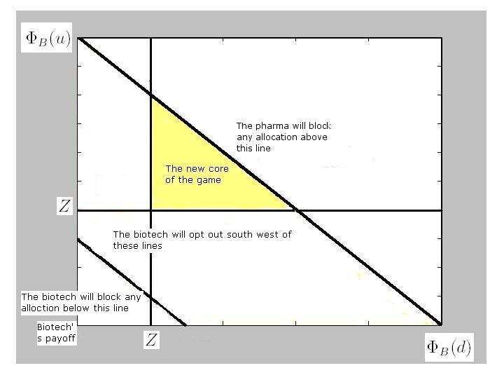
4.3 The core of an options contract: an illustrative model Figure 4.1: The core of the cooperative game with the biotech having the opt-outoption 2. The opt-out lines intercept in the core (x∗ ≤ Z ≤ x∗ ). This is depicted in figure For this to happen Z has to be more than the payoff of the downside but less than the payoff in the upside. The change in the core is in favour of the option owner, i.e. the option improves the option holder's 3. The opt-out lines intercept above (northeast of) the core (Z ≥ x∗ this case the core is empty. This happens only if the opt-out payoff Z exceeds the payoff in the upwards scenario.
The above relationships between Z and the payoff core translate to the rela- tionships developed in section for the relationship between Z and the value core in the complete markets case.
The effect of risk aversion Having dealt with the situation of hedging in complete markets and of risk-neutral agents in the absence of markets, we will now discuss an arguably more realistic situation where we assume that the agents are risk averse with possibly different 4.3 The core of an options contract: an illustrative model levels of risk aversion. This is a sensible assumption for example in partnership negotiations between pharma majors and relatively small biotechs. As pharma majors are well-diversified and well endowed pharma they are almost risk neutral.
In contrast, relatively small biotech companies have serious cash constraints and due to the fact that they rarely have drug candidates close enough to the market to raise additional equity capital, tend to be risk averse. We assume that there are no partial hedging opportunities. The presence of possibly different levels of risk aversion introduces two interesting issues: 1. If two players have different levels of risk aversion they should be willing to trade off risk. This raises the question of how risk could be shared in an 2. If two players have different levels of risk aversion, they may well come to different conclusions about the most desirable contract design. A risk averse partner might be willing to pay the costs associated with waiting in order to have an option that will reduce her risk - a less-risk averse partner might not agree. How can these differing preferences be reconciled? We address the first issue in section where the agents have only one possible project design available. We introduce the problem of design choice in section where agents can choose to set up cooperative options or not. In section we discuss the effect of non-cooperative options.
Cooperative games and risk aversion We will illustrate the risk sharing issues using our simple two agent partnership contract, without any options. This section, which is largely based on sets the scene for the analysis of options effects under risk-aversion.
We assume, as before, that the stochastic payoff X is modelled as a flip of a possibly biased coin. The two agents have different attitudes towards risk: the biotech is more risk averse than the pharma. We model their payoff preferences via expected utility functions Since we assume that the agents' perceptions of risk 1Agent i prefers an uncertain payoff X over an uncertain payoff Y if E[ui(X)] > E[ui(Y )], where ui is a suitable utility function.
4.3 The core of an options contract: an illustrative model Figure 4.2: Efficient risk sharing are fully captured by an expected utility, it is possible to gauge how much a risky gamble would be worth to each player: Given a gamble X, what deterministic payment mi would make agent i indifferent to receiving mi for sure or taking the gamble? This value is the certainty equivalent of the risky gamble; it satisfies ui(mi(X)) = E[ui(X)], i.e. mi(X) = u−1(E[u i(X )]). For illustrative purposes we choose exponential utility functions: u βP > βB.
What is the optimal way for the companies to share the risk involved in a joint project? We will focus on linear contracts, i.e. agreements involving a deterministic payment Di and a share ri of an uncertain payoff X. The total payoff of agent i from the joint project will be Φi(ω) = Di + riX(ω).
Such simple royalty contracts are commonplace in business, in particular in licensing agreements in the pharmaceutical industry. This type of contract is 4.3 The core of an options contract: an illustrative model illustrated in figure where we wish to determine an allocation along the diag- onal in the space of state-payoffs. The closer the agreement point is to the origin, the more risk is taken up by the biotech and the less risk by the pharma. In the case of risk-neutral companies the utility indifference curves are straight lines. If agents are risk averse then the indifference map is no longer linear as can be seen Both agents prefer to take up as little risk as possible. However, the risk aversion induced by the concave utility function reduces the marginal benefit of a decrease in risk taking. Furthermore, this rate of reduction of marginal benefits will be different for both players in view of their differing risk aversion levels. The royalty rate r that maximises the perceived total vaof the game is achieved where the marginal value of taking up some infinitesimal fraction of the risky project is the same for both agents. If the marginal benefits were different we would be able to add to the total value by taking away an infinitesimal amount of risk from the player with the smaller marginal benefit and giving it to the player with the larger marginal benefit. This can be seen in figure Formally, the agents solve the maximisation problem XB+P = max mB(ΦB(ω)) + mP (ΦP (ω)) where (ΦB, ΦP ) are given by equation with X(ω) = ωCB+P − IB+P , ω ∈ {u, d} This is a standard problem in the risk sharing literature where it is a well known fact that for HARA utility functions linear contracts can be an efficient risk sharing tool. In the next paragraph we show that linear contracts are efficient sharing tools in a cooperative game with options.
1In the context of a partnership players cooperate to maximise the total value of the con- tract. We model this objective by assuming that the players wish to maximise the sum of theircertainty equivalents.
4.3 The core of an options contract: an illustrative model Under our assumption of an exponential utility function we have m(D + Y ) = D + m(Y ) for any deterministic payoff D and stochastic payoff Y . The problem therefore reduces to XB+P = max (mB(rBX) + mP (1 − rB)X)) with a first order optimality condition P ((1 − rB )X ) .
For the exponential utility function the optimal share of risk for each player is proportional to their risk tolerance Although this condition specifies how much risk each player will take, it does not determine the total payoff.
This is because the deterministic amount D that agents exchange is not constrained and is determined in negotiation. The stochastic cooperative game is again reduced to a deterministic game with a value core in the standard sense.
The core of the game, subject to optimal risk sharing, is now specified by the following conditions mB(rBX(ω)) + DB ≥ XB mP (rP X(ω)) + DP ≥ 0 , i ∈ {B, P }.
where XB = mB(ωCB − IB) with ω ∈ u, d. The first two conditions guarantee that each agent's estimation of the value is at least as good as going it alone.
The third condition is a conservation law: the total amount that changes hands is zero and the forth condition will ensure efficient risk sharing. The value core is 4.3 The core of an options contract: an illustrative model again one-dimensional, involving only the deterministic amounts Di that the two companies will exchange XB − mB(rBX(ω)) ≤ DB ≤ mP (rP X(ω)), and DP = −DB.
It is interesting to consider the special case when CB = CB+P , IB = IB+P and sB = sB+P . In this case there are no synergies in the traditional sense. It is not surprising that when the agents are risk-neutral the only core allocation for the biotech is φB = CB − IB. Nothing is gained by a partnership. However, if agents are risk averse, cooperation is valuable. It can be seen from equation that the core has a non-empty interior. In other words, there are gains to be made by cooperating, because of risk sharing. The corresponding risk sharing set can be thought of as the pure risk sharing core of the contract XB − mB(rB[ωCB − IB]) ≤ DB ≤ mP (rP [ωCB − IB]).
An interesting observation can be made here. As the risk preferences of the two companies diverge (βB << βP ), it is optimal for the pharma to take a larger amount of risk (rB → 0, rP → 1). As can be seen from equation the risk sharing core of the deal is enlarged:. Therefore risk sharing synergies become more valuable.
To summarize, the presence of risk aversion does still allow for the reduction of the stochastic cooperative game to a deterministic game, just as in the previous section. Suitable linear sharing rules are Pareto-efficient, see and allow an optimal risk sharing. Once the agents agree that they wish to share risk optimally, the cooperative game is played on the deterministic amount that the agents will exchange.
Cooperative options and risk aversion To illustrate the issue of disagreement on contract design, let us revisit the ex- ample of the cooperative option. As before, we suppose the agents have to decide 4.3 The core of an options contract: an illustrative model whether or not to pay amount kB, or kB+P in partnership, up front in order to postpone the launch decision until uncertainty is resolved.
In this situation the value of the joint project with the option becomes Xi = mi(ωCB+P − IB+P )+ − kB+P .
Note that this is agent i's personal valuation of the joint project. For different levels of risk aversion it is possible that the agents will order the two designs differently and would disagree which design to choose in a partnership.
In the presence of complete markets the partnership would choose the design with the highest no-arbitrage value. In the present situation it would seem sen- sible to assume that the coalition will choose the project design that maximizes the total certainty equivalent for the coalition, provided that they share the risks If the biotech develops the project alone it has to choose between not investing in the option, which has value XB = mB(ωCB − IB), or investing in the option, which has value X B ((ωCB − IB )+ − kB ). Similarly, the partnership has a choice between XB+P given in and B (ΦB (ω)) + mP (ΦP (ω)) where (ΦB, ΦP ) are given by equation with X(ω) = (ωCP +B − IB+P )+ − kB+P , ω ∈ {u, d} and the probability of event u is p.
Assuming that it is optimal for the partnership to set up the option, i.e.
B+P , the core of the game becomes a negotiation over the payments 1For our example of exponential utility functions the risk sharing rule only depends on the risk tolerance βi of each player and not on the distribution of the gamble payoffs. Therefore,we do not need to solve the optimal risk sharing problem again; it is the same as before withsolution ri = . For other forms of HARA utility functions, such as logarithmic or power law utilities, the optimal share of risk for each agent depends on the payoff at each state and,therefore, would be different in the presence of flexibility.
4.3 The core of an options contract: an illustrative model mB(ΦB(ω)) + DB ≥ max{XB, X } mP (ΦP (ω)) + DP ≥ 0 Φi(ω) = ri((ωCB+P − IB+P )+ − kB+P ) As before, the core of the cooperative options game can be expressed in terms of the fixed amounts DB that is exchanged max{XB, X } − m B (ΦB (ω)) ≤ DB ≤ mP (ΦP (ω)).
Similarly to the risk-neutral case, the asset value of the contract is the core of the contract in the absence of flexibility and the option value is the added value from flexibility. Each of these values has a risk sharing component in the sense that if the partnership does not have any synergies other than risk sharing, both the asset and the option cores are non-empty.
Non-cooperative options Let us now revisit our example of unilateral flexibility in the context of risk- aversion. To simplify the exposition we assume that there are no cooperative options. As before, we assume that the biotech has the right to opt out of co- marketing. However, here we will consider a more general opt-out agreement where the biotech receives a fixed amount Z (milestone payment) and royalties rRCB+P on the revenue CB+P if the option is exercised. The biotech company can exercise this option after uncertainty is resolved and, assuming a linear risk- sharing agrement as before, would do so if and only if rB(ωCB+P − IB+P ) + DB ≤ Z + rRωCB+P where rB is the biotech's share of the revenues from co-marketing and ω ∈ {u, d} is the current state of the world at exercise. The problem of finding an optimal risk sharing arrangement now becomes: 4.3 The core of an options contract: an illustrative model mB(max{rBX(ω) + DB, Z + rRωCP +B}) +mP (min{rP X(ω) + DP , X(ω) − rRωCP +B − Z}) DB + DP = 0.
In this case, the computation of the optimal royalty value and the determin- istic payoff are not decoupled. The optimization is a non-smooth non-convex problem, due to the max and min terms in the objective function. Furthermore, we are no longer guaranteed to find an optimal linear risk sharing rule.
One way to avoid these complications is to require rR = rB, i.e. the royalty rate is independent of the options exercised and set at the optimal level for the game without the unilateral option, as explained in the previous section. By doing this, we allow the biotech to opt out unilaterally but we do not affect the efficient risk allocation. As a result, the non-cooperative option will be exercised only if the amount Z, the milestone, is higher than the amount DB the biotech receives from the pharma if it does not opt out. The core now satisfies the following mB(rBX(ω)) + max(DB, Z) ≥ mB(ωCB − IB) mP (rP X(ω)) + min(DP , −Z) ≥ 0 , i ∈ {B, P }.
Solving for DB gives the reduced representation max{Z, mB(X(ω)) − mB(rB(ωCB+P − IB+P ))} ≤ DB ≤ mP (rP (X(ω))) Similarly to section we can distinguish three cases depending on the value of Z and the associated exercise decisions.
4.4 Cooperative real options games in continuous-time Cooperative real options games in continuous- In this section we will show how the model developed in section can be generalized to games with continuous-time dynamics and multiple agents. We will focus on cooperative real options games with the following schedule of events 1. At time t = 0 the agents decide which coalition to form and the coalition decides which contract design to choose.
2. At time t = T the coalition observes uncertainty and decides on the exercise of any available cooperative options.
3. Payoff is instantly realized and shared.
Non-cooperative options, if they exist, are exercised immediately after the exercise of the cooperative options. Our goal is to provide guidance on fair and sensible Our setting assumes a European options framework, where optimal timing of the exercising of the options is not an issue. Extending the formulation of a stochastic cooperative game, see we formally specify a Eu- ropean cooperative options game as a probability space (Ω, F, P) with a filtration{Ft}t≥0 and a tuple (N, AS, BS, XS), where • N is a finite set of agents • AS are the sets of contract design choices available to the coalitions S ⊆ N at time t = 0, before uncertainty is resolved • BS(a, ω) are the sets of actions available to the coalitions S ⊆ N at time t = T , provided S has chosen design a ∈ AS at time t = 0 and the event ω ∈ Ω occurs; these are the options available to the coalition • XS(a, b, ω) are the payoffs to the coalitions S at time t = T , provided the coalition has chosen to implement design a ∈ AS and has exercised the option b ∈ BS(a, ω) after the event ω ∈ Ω occurred 4.4 Cooperative real options games in continuous-time Cooperative options in complete markets We begin with a discussion under a complete markets assumption which will allow us to use standard arbitrage pricing arguments, see for example for details. We assume that there is a complete arbitrage-free market of traded assets.
This is equivalent to the existence and uniqueness of a martingale measure Q forthe market such that any claim X(T ) has a no-arbitrage price of x = EQ[e−ρT X(T )], where ρ is the risk-free rate, see In particular the coalition payoffs XS(a), following optimal options exercise strategy at t = T , can be priced in this way as xS(a) = EQ[e−ρT XS(a, b, ω)].
The value xS(a) is called the risk-neutral valuation of the payoff to coalition S. Given design a ∈ AS and state ω ∈ Ω, a coalition S will choose the action b∗ (a, ω) ∈ B S (a, ω) that maximizes its payoff XS (a, b, ω).
Since all uncertainty has been resolved this is a deterministic optimization decision, resulting in a contingency plan b∗ for coalition S.
Under our assumptions, the risk-neutral value xS is the only value that is consistent with the observed asset prices in the sense that it does not allow for arbitrage profits through trading. The coalition can sign the contract a and at the same time short-sell the associated replicating portfolio. This will result in an immediate payoff of xS(a) and no future payoff when uncertainty is resolved because the replicating portfolio, suitably re-balanced during the trading period [0, T ], will hedge all future payoffs from the contract. The coalition then uses the risk-neutral valuation to choose the design a∗ ∈ A S that maximizes the total risk xS = max xS(a).
Given the optimal design choices a∗ and contingency plans b∗ (a∗ , .), the real 4.4 Cooperative real options games in continuous-time options game reduces to a deterministic cooperative game Γ = (N, {xS}S⊆N ).
Cooperative game theory is primarily concerned with payoff sharing rules Φ(ω) = (Φi(ω), i ∈ N ), where Φi(ω) specifies the payoff for agent i if state ω ∈ Ω has occurred. The sharing rule has to satisfy X Φi(ω) = XN(a∗, b∗ (ω), ω), ∀ω ∈ Ω.
The reduced deterministic game Γ, however, is specified in terms of risk-neutral values xS, not in terms of final coalition payoffs. The focus shifts from payoff allocations Φ(ω), specified for each future state ω ∈ Ω to value allocations φ = (φi, i ∈ N ), where φi is agent i's share of the total value xN . A payoff sharing rule Φi(ω) for agent i is compatible with a value allocation φi if φi = EQ[e−ρT Φi(ω)].
In view of the complete markets assumption, agent i can always achieve the value φi associated with a payoff sharing rule Φi by shorting the replicating portfolio for Φi. This will result in an immediate payoff φi and no future payoffs. The discussion of sensible sharing arrangements has moved from the space of functions Φ : Ω → RN to the space of vectors φ ∈ RN .
The complete markets assumption is frequently made in the literature, see for example although it is rather restrictive. The above analysis remains conceptually correct in a situation without hedging opportunities, provided the agents are risk-neutral and the following conditions apply: • The martingale measure Q is replaced by the, possibly subjective, proba- bility measure P of the underlying probability space and agents have ho-mogenous beliefs about this 1If agents have heterogenous beliefs efficient side betting may be employed, see 4.4 Cooperative real options games in continuous-time • The agents agree on a suitable discount rate ρ.
Notice that in the absence of a complete market, the payoff sharing rule Φ(ω), ω ∈ Ω, needs to be specified in the contract, because agents cannot hedge their risks through shorting a replicating portfolio. However, if all agents are risk neutral then they will be indifferent between payoff allocations that result in the same value φ. For example one agent may receive the stochastic payoff XN (a∗, b∗(ω), ω), taking all the risk, and pay all other agents their deterministic value share φi.
We will deal with the more interesting risk-averse case in the absence of a market Since the cooperative real options game in a complete market reduces to the deterministic cooperative game Γ we can apply the standard solution concepts of cooperative game theory to the value sharing agreements φ, see for example The value-core of the game consists of all allocations φ = (φi, i ∈ N ) such that no sub-coalition S can receive more value from going alone, i.e., All payoffs are allocated to the agents in the grand coalition N , i.e.
The Shapley value φi of agent i is calculated as the Shapley value of the deterministic reduction Γ X S !(N − S − 1)! We close this section with two illustrative examples of what one may call the Black-Scholes-Shapley value, which results when the standard Black-Scholes assumptions apply.
Example 1. Consider a game with three agents.
4.4 Cooperative real options games in continuous-time 1. The first agent owns a project with stochastic payoffs with present value X0. The value follows a geometric Brownian motion with volatility σ2. The agent will have to sell the project at time T for the then market price XT .
2. The second agent can offer an expansion option to the project. This call-like option will cost kC to set up, has an exercise cost (strike price) of KC and can only be exercised at time T . The Black-Scholes value of this European C = X0Φ(d1) − KCe−ρT Φ(d2), where Φ(x) is the standard normal cumulative distribution function, d1 = 2 = d1 − σT .
3. The third agent can offer an abandonment option to the first agent. This put-like option will cost kP to set up, offers a sure payment KP < KC if exercised, and can again only be exercised at time T . The Black-Scholes value of this option is P = KP e−ρT Φ(−d2) − X0Φ(−d1).
The design set A{1,2,3} for the grand coalition contains four designs: no option, the call option only, the put option only, or both options. Set A{1} has only one design: no option, sets A{2},A{3},A{2,3} are empty and sets A{1,2} and A{1,3} have two obvious elements of no option or the option that the respective partner brings to agent 1. The optimal design for this problem is to include an option if its risk- neutral value exceeds its set up cost, i.e. C ≥ kC or P ≥ kP , respectively.
The optimal exercise strategy for the options is to exercise the call option if the price XT ≥ KC and to exercise the put option if XT ≤ KP . The Shapley-value φ = (X0 + (C − kC)+ + (P − kP )+, (C − kC)+, (P − kP )+).
This allocation is very intuitive; the first agent receives the whole value of his project and half the option value added by each of the other two agents. The 4.4 Cooperative real options games in continuous-time other two agents receive half the value of the option they bring to the deal. The following example is less intuitive.
Example 2. Again we consider three agents.
1. The first agent owns the same project as in Example 1.
2. The second agent can offer both an expansion and an abandonment option to the project at costs kC and kP , strike prices KC and KP and values C and P respectively. The Black-Scholes values C and P are given by the respective formulas in the above example.
3. The third agent can lower the strike price for the call option to K0 < K and can increase the strike price of the put option to K0 > K K0 > K0 ), without any additional costs, therefore increasing the value of the two options to C0 and P 0.
Now the design sets A{1,2,3} and A{1,2} contain four designs: No options, the call alone, the put alone, and both options. Sets A{1} and A{1,3} only contain the no-option design, sets A{2},A{3},A{2,3} are empty. As before, the optimal design is to include an option if its risk-neutral value exceeds its set up cost, i.e., C ≥ kC or P ≥ kP or C0 ≥ kC or P 0 ≥ kP . Assuming it is optimal to include all options, the Shapley-value allocation is φ3 = (C0 + P 0) − (C + P ).
There is no straightforward intuitive explanation for this Shapley-value allo- Unilateral options in complete markets We will now add the possibility that one agent, say agent i, owns a unilateral option. The timing is now as follows: 4.4 Cooperative real options games in continuous-time 1. At time t = 0 the agents decide which coalition to form and which contract design to choose.
2. At time t = T the coalition observes uncertainty and decides how to exercise the available options.
3. Agent i decides how to exercise her options unilaterally, immediately after the exercise decision for the cooperative options.
4. Payoff is instantly realized and shared.
To simplify notation we will ignore discounting for the remainder of this section.
Suppose agent i has the option to leave the partnership for an agreed de- terministic payoff Z once uncertainty is resolved. Such an option will only be exercised in states ω where Z exceeds the payoff Φi(ω) the agent would receive in the partnership after the resolution of uncertainty and the exercise of the co- operative options.
Were we will make a few observations, which will be stated in the form of Proposition 17 The unilateral option does not change the total value of the contract for any coalition.
Proof Assume that Φi is the option owner's agreed share of the payoff before the unilateral option is exercised. The value of the contract to the option owner is then φi = EQ[max{Φi(ω), Z}] while the sum of the value to everyone else in a coalition S with agent i is the residual value φS−i = EQ[XS(ω) − max{Φi(ω), Z}].
Here we have used the fact that Φ(ω) satisfies P i(ω) = XS (ω). The total value to the coalition S is therefore φS = φi + φS−i = EQ(XS(ω)) = xS, which is independent of the option.
Proposition 18 The value share of the option owner satisfies φi ≥ Z indepen-dently of the payoff sharing arrangement.
4.4 Cooperative real options games in continuous-time Proof Let Φi(ω) be the payoff sharing rule for the agent who owns the non- cooperative option. Then her value will satisfy φi = EQ[max{Φ(ω), Z}] ≥ EQ[Z] = Z.
Proposition 19 The opt-out option changes the value core to max{xi, Z} ≤ φi φj ∀S ⊆ N, S 6= {i} where i is the owner of the non-cooperative option.
Proof Recall the conditions of the value core of the game without the unilateral option. The first inequality in the proposition follows immediately from Proposition and the inequality for S = {i}. The constraints in for coalitions S : i / ∈ S, S ⊆ N are not affected by the presence of the non-cooperative option since the owner of the option is not a member of these coalitions. Due to Proposition the core conditions for coalitions S : i ∈ S, S 6= {i}, S ⊆ N are also not affected.
Proposition has some interesting consequences. At first glance it seems difficult to assess what the added bargaining value of the opt-out option is for its owner. The option adds value for its owner, provided there exists states ω ∈ Ω with positive probability such that the payoff Φ(ω) < Z. This however, requires an agreed payoff sharing rule in the first place. Proposition shows that the value core remains independent of the payoff sharing rule. A comparison with the value core without the unilateral option shows that the option adds bargaining value to its owner agent i only if Z > xi.
Traditional real options wisdom has it that an option always has a non- negative value for its owner. Proposition however, shows that this is not necessarily the case for non-cooperative options in a partnership. If the value of the option is more than the agent's contribution to the coalition (Z > xN − xN−i) 4.4 Cooperative real options games in continuous-time then the core becomes empty. The option destroys the partners' incentive to forge a deal and consequently, the unilateral opt-out option will not be realized.
The foregoing results for unilateral options can be extended to opt-out options owned by coalitions S ⊆ N . If O is the collection of coalitions S that have non-cooperative opt-out options with payoff ZS then the conditions for the value core max{xS, ZS} ≤ φS = Proposition 20 For every value allocation in the core there is a payoff allocation such that the unilateral option is never exercised.
Proof. Let φ = (φj, j ∈ N ) be an allocation in the value core and Φ = (Φj, j ∈ N ) be an associated payoff allocation. Then  = φi − Z ≥ 0 in view of Proposition If agent i owns the option and we define the new payoff allocation i(ω) − Z −  then the corresponding value allocation satisfies = EQ[Φj(ω) + Φi(ω)−Z− ] = EQ[Φj(ω)] + EQ[Φi(ω)]−Z− = EQ[Φj(ω)] + φi−Z− Φ(ω) = XN (ω).
4.4 Cooperative real options games in continuous-time Hence the allocation ˜ Φ is in the payoff core and corresponds to a value allocation φ. The unilateral option will not be exercised because ˜ Φi(ω) ≥ Z for all ω.Q.E.D.
The condition φi ≥ max{xi, Z} in Proposition shows that the non-cooperative option provides a second participation benchmark, in addition to the go-alone value xi, for its owner. The threat of exercising the option is just as credible as the threat of breaking away from a coalition because the go-alone value is larger.
Proposition is interesting in this regard because it shows that non-cooperative options are powerful bargaining tools, even though the agents may be able to avoid their exercise through a suitable payoff sharing arrangement. This is remi- niscent of the fact that the threat of leaving the coalition is a powerful tool that is not exercised, provided the agent's share is in the value core.
An interesting case, not covered by the discussion above, occurs if a unilateral option depends on an exogenous uncertainty, i.e. an uncertainty that adds value to the option owner but is not part of the contract. In such cases the options owner may well exercise the non-cooperative option sub-optimally with regard to the deal but optimally with regard to her overall objective. For example, a biotech company may opt out of a co-development contract because some other project in their portfolio, not covered by the contract, is very promising and it makes sense for them to redirect the funds Z from the contract to the external project. In such circumstances it is possible that the non-cooperative option will add value to a coalition as a whole and not only to its owner. A study of such options effects would be interesting but is beyond the scope of this paper.
Risk aversion in the absence of hedging opportuni- We will next consider a situation where risk averse agents negotiate a partnership contract without hedging opportunities through traded assets. We model risk aversion through utility functions ui, which we assume to have hyperbolic absolute risk aversion (HARA) in order to be able to use the fact that linear contracts are efficient, see Prominent examples of HARA utility functions are exponential utilities ui(x) = ai exp(bix), bi, ai < 0 (constant absolute risk aversion), power law utilities ui(x) = aixbi, ai > 0, 0 < bi < 1 (constant relative 4.4 Cooperative real options games in continuous-time risk aversion) and, the limiting case as bi → 0, logarithmic utilities ui(x) = Agent i's certainty equivalent of a stochastic payoff X at time T is the amount mi(X) that would make the agent indifferent between receiving mi(X) for sure at time t = 0 or receiving the stochastic payoff X at time t = T . Formally, mi(X) = u−1(E[u where ρ is the risk-free discount rate.
We assume that the timing of the cooperative game is as before: agents agree on the coalition and an options design at t = 0. Then, after uncertainty is resolved, they decide on the options exercised at t = T and receive an instant There are two complications compared to the complete markets case: • In the complete markets case the final payoff sharing rule Φ(ω) is irrelevant because of the presence of the replicating portfolio and associated hedging of risks. Sharing happens at the level of risk-neutral values. In the present case, the coalition needs to specify an explicit payoff sharing rule, taking account of the agents' risk-aversion.
• Due to possibly differing risk preferences, the agents in a coalition S might not agree which design a ∈ AS they prefer. To overcome this problem, we will assume that a coalition S makes decisions in the interest of maximizing the sum of the certainty equivalents mi of the agents i ∈ S.
We will make use of the theory of linear contracts and efficient risk sharing in the development of the model. In a linear contract, each agent i in a coalition S receives a deterministic payoff Di before uncertainty is resolved and a proportion ri of the risky payoff XS(a, b, ω), i.e. its payoff allocation is of the form Φi(ω) = Di + riXS(a, b, ω).
4.4 Cooperative real options games in continuous-time To achieve complete sharing we assume that the deterministic payoffs Di and royalties ri satisfy ri = 1, ri ≥ 0 ∀i ∈ S.
As mentioned above, we will also assume that coalitions act in the interest of maximising the sum of the certainty equivalents of their members. Applying this principle to the admissible contracts (Di, ri) will ensure Pareto-efficiency. The corresponding total value for a given design a ∈ AS is given by mi( max [Di + riXS(a, b, ω)]) subject to the constraints Note that the risk averse agents will always agree which of the options b(a, ω)∗ ∈ BS(a, ω) to choose because all uncertainty is resolved at the time of exercise. Also, this exercise policy is independent of the royalty rate ri.
The optimization problem decouples if which is the case for exponential utilities. Under this assumption the optimization mi(riXS(a, b∗(a, ω), ω)).
Pi∈S ri=1 i∈S The deterministic shares Di are inconsequential to this optimization problem.
Optimal royalty rates r∗ are chosen from the simplex and hence exist if the functions fi(r) = mi(rXS(a, b∗(ω), ω)) are continuous and are unique if these functions are strictly concave, e.g. in the case of exponential utilities. If the functions fi are differentiable then the optimal rates are characterized by the 4.4 Cooperative real options games in continuous-time i > 0, rj > 0 ≥ ∂fj(rj) if r If does not hold then the optimal allocations (ri, Di) have to be computed simultaneously. With gi(Di, ri) = mi(Di + riXS(a, b∗(ω), ω) the KKT conditions i > 0, rj > 0 ≥ ∂gj(Dj,rj) if r Given the optimal allocation (ri, Di) for coalitions S and option designs a ∈ AS, the coalition can now decide on the best design a∗ ∈ AS. This results in the value XS = max[XS(a)].
The stochastic game with real options is therefore again reduced to a deter- ministic cooperative game assuming that the agents choose the design a∗, exercise the options b∗(a∗, ω) and each agent takes a proportion r∗(a∗) in the risky payoffs. As in the complete markets case, the standard solutions concepts of cooperative game theory apply.
A key assumption for the model is that the agents in a coalition S agree on a measure of total contract value associated with a given payoff sharing rule (Di, ri) and a design a ∈ AS. Here we have assumed that this total value is measured by the sum of the certainty equivalents. Similar models can be developed if total contract value is measured by a, possibly suitably weighted, sum of expected 4.4 Cooperative real options games in continuous-time Non-cooperative options and risk aversion Let us finally turn to non-cooperative options. We assume that non-cooperative options are exercised instantly after the exercise of the cooperative options, if there are any. Whilst the general principles of the former section are transferable, it now becomes considerably more difficult to analyse options effects. The chief reason is that the unilateral options exercise will typically turn the certainty equivalents of the players into nonsmooth and possibly nonconcave functions. As a consequence, it might no longer be possible to split the risk efficiently in a linear way amongst the agents.
Assume, for example, that agent i can opt out and receive a fixed amount Z after uncertainty is resolved. Her payoff from the project if design a ∈ AS is Φi(ω) = max(Di + riXS(a, b∗(ω), ω), Z), where b∗(ω) captures the contingency plan for the exercise of the cooperative option, prior to the exercise of the non-cooperative opt-out option. The cer- tainty equivalent mi(Φi(ω)) is now a nonsmooth function of ri at the points where it becomes optimal to opt-out. As a result, the certainty equivalent of all other players is nonsmooth at these points. The optimal risk- sharing is non-linear because it is contingent on opt-out. The players j ∈ S {i} will have to agree on risk sharing rules for both cases, these being that player i either stays in or opts out.
There is a possible way out of this dilemma. Instead of paying a fixed de- terministic payment on opt-out, we pay agreed royalties and milestones, i.e. an agreed royalty rate rO on the uncertain payoff plus a fixed payment Z. Deals of this type are commonplace, e.g. in drug licensing. The royalties force the option owner to retain some of the risk, even if she has exercised the opt-out option.
If we choose rO to be the optimal rate for the case without the non-cooperative option, then optimal risk sharing between the agents is maintained. The payoff to the option owner is now max(Di, Z) + riXS(a, b∗, ω). The option will only be exercised if Z > Di. The core is shifted in favour of the option holder, similarly to the complete markets case.
4.5 Managerial implications and conclusions Managerial implications and conclusions We have drawn attention to sources for partnership synergies beyond the tradi- tional economies of scale and scope. Our focus is on synergies in the presence of uncertainty, in particular risk sharing opportunities when partners have different attitudes towards risk and the value of flexibility within a partnership.
Our models provide three main managerial insights. First of all, partners with divergent risk attitudes gain more synergies from risk sharing in uncertain envi- ronments. Teaming up with a partner with a different risk attitude can be very beneficial in this regard. Risk sharing opportunities increase both the asset core, i.e. the synergy set from traditional economies of scale and scope, as well as the options core, i.e. the set of synergies gained from flexibility. A prominent exam- ple of where risk sharing synergies are particularly relevant are co-development contracts between pharma majors and smaller biotechnology companies.
Secondly, what can a company do to improve its bargaining position? Improv- ing the bargaining position is equivalent to shifting the synergy set to a region of higher individual payoff or, in the risk-averse case, higher individual utility. This can be accomplished in several ways. Companies can aim to improve their go- alone capability, either through the traditional ways of improving the efficiency of operations or by increasing out-of-the-deal opportunities. Alternatively, a com- pany could increase the volatility that underlies its flexibilities, e.g. by improving its pipeline of innovative but high-risk projects. Finally, non-cooperative options, negotiated prior to a deal, can shift the synergy set in favor of the option holder.
Thirdly, non-cooperative options are a double-edged sword. On the one hand they are valuable for individual partners because they cut off lower utility parts of the core. However, if partners are too greedy in setting non-cooperative options clauses then this can make the core empty. Partnerships that still go ahead are more likely to fail when the locked-in partner realizes the pitfalls of giving away From an academic point of view, this paper provides a framework for the investigation of partnership deals in the presence of uncertainty and flexibility.
The models are illustrative and stylized but provide the basis for interesting insights. There is much scope for future work. We only mention four areas: 4.5 Managerial implications and conclusions 1. We have focused on European options in this paper. It would be interesting to extend the framework to American options where the partners have to agree on optimal exercise policy of joint options as well as a profit sharing rule. Given that there is an option exercise strategy that maximizes the total project value, it might be possible to come up with a profit sharing rule that enforces it. demonstrates that this is the case for mergers motivated by economies of scale. He finds that there is a unique post-merger ownership rule that synchronizes the option exercise policy at the first best. This is possible because the economies of scale make the problem convex. In our setting, the convexity that permits one solution comes from the risk aversion.
2. We have focused on two extreme situations - complete markets on one side and no markets but risk aversion on the other. What if there are partial hedging opportunities? The work of on the integra- tion of decision analysis and real options valuation would be an interesting starting point for investigations in this direction.
3. We have focused on a closed contract world. Most companies have invest- ment opportunities outside of the contract and therefore will not necessarily exercise their contractual options in the interests of the underlying contract project. This can lead to some interesting effects when unilateral options are exercised optimally within a company's portfolio of opportunities but sub-optimally within the contract frame.
4. We have focused on sequential decisions by the partners. If we allow for simultaneous decisions then we are in the context of a cooperative game fol- lowed by a non-cooperative game - cooperate to compete is the sequencing.
Work along these lines should provide an interesting angle to the study of the relationship between cooperation and competition in the strategy field, see and would complement recent work by on biform games.
4.5 Managerial implications and conclusions Last but not least, we believe that there are ample opportunities out there fore the theories developed in this paper to have a practical impact on business. A coop- erative real options framework can be useful in helping companies understand the value effects of contingency clauses and can thereby help them structure more effi- cient and more robust contracts. We have had some practical experience with our developed concepts during the negotiations of a complex co-development contract which included substantial flexibility, between Cambridge Antibody Technology Plc., a UK-based biotech company, and Astra ZeWhilst this experience was encouraging, it also revealed that much work remains to be done in order to make cooperative real options models useful on a broad scale in business practice.
Adner, R., D.A. Levinthal. 2004a. Real options and real tradeoffs. Academy of Man- agement Review 29 120–126. Adner, R., D.A. Levinthal. 2004b. What is not a real option: Considering boundaries for the application of real options to business strategy. Academy of Management Review 29 74–85. Black, F., M. Scholes. 1973. The pricing of options and corporate liabilities. Journal of Political Economy 81(3) 637–59. Bowman, E.H., G.T. Moskowitz. 2001. Real options analysis and strategic decision making. Organization Science 12 772–777. Brandenburger, A., H. Stuart. Forthcoming. Biform games. Management Science . Brandenburger, A.M., B.J. Nalebuff. 1996. Co-opetition. Harper Collins Business, Brennan, M.J., E.S. Schwartz. 1985. Evaluating natural resource investents. Journal of Business 58 135–157. Burnetas, A., P. Ritchken. 2005. Option pricing with downward-sloping demand curves: The case of supply chain options. Management Science 51(4) 566–580. Christensen, P., G. Feltham. 2002. Economics of Accounting, vol. 1. Kluwer Academic Dixit, A., R. Pindyck. 1994. Investment under uncertainty. Princeton University Press.
Granot, D. 1977. Cooperative games in stochastic characteristic function. Management Science 23(6) 621–630. Grenadier, S. 2002. Option exercise games: an application to the equilibrium investment strategies of firms. The Review of Financial Studies 15(3) 691–721. Harrison, M., S. Pliska. 1981. Martingales and stochastic integrals in the theory of continuous trading. Stochastic Processes and their Applications 11 215–260. Hull, J.C. 2003. Options, Futures AND Other Derivatives. 5th ed. Prentice Hall. Kogut, B. 1991. Joint ventures and the option to expand. Management Science 37 Kulitilaka, N., E.C. Perotti. 1998. Strategic growth options. Management Science 44 Lambrecht, B.M. 2004. The timing and terms of mergers motivated by economies of scale. Journal of Financial Economics 72(1) 41–62. McGrath, R.G. 1997. A real options logic for initiating technology positioning invest- ments. Academy of Management Review 22 974–996. McGrath, R.G. 1999. Falling forward: Real options reasoning and entrepreneurial failure. Academy of Management Review 24(2) 12–30. McGrath, R.G., W.J. Ferrier, A.L. Mendelow. 2004. Real options as engines of choice and heterogeneity. Academy of Management Review 29 86–101. McGrath, R.G., A. Nerkar. 2004. Real options reasoning and a new look at the R&D investment strategies of pharmaceutical firms. Strategic Management Journal 25 Merton, R.C. 1973. Theory of rational option pricing. Bell Journal of Economics and Management Science 4 141–181. Myers, S.C. 1984. Finance theory and financial strategy. Interfaces 14 126–137. Nash, J. 1950. The bargaining problem. Econometrica 18 155–162. Nash, J. 1953. Two person cooperative games. Econometrica 21 128–140. Pratt, J. 2000. Efficient risk sharing: The last frontier. Management Science 46(12) Rivoli, P, E. Salorio. 1996. Foreign direct investment and investment under uncertainty.
Journal of International Business Studies 27 335–357. Shapley, L.S. 1953. A value for n-person games. A.W Kuhn, H.W. Tucker, ed., Con- tributions to the Thoery of Games II . Princeton University Press, 307–317. Sharpe, W. 1995. Nuclear financial economics. W. Beaver, G. Parkter, eds., Risk Management: Challenges and Solutions. McGraw-Hill, 17–35. Smith, E.J., R.F. Nau. 1995. Valuing risky projects: Option pricing theory and decision analysis. Management Science 41(5) 795–816. Suijs, J., P. Borm. 1999. Stochastic cooperative games: Superadditivity, convexity, and certainty equivalents. Games and Economic Behavior 27(2) 331–345. Suijs, J., P. Borm, A. De Waegenaere, S. Tijs. 1999. Cooperative games with stochastic payoffs. European Journal of Operational Research 113(1) 193–205. Wilson, R. 1968. The theory of syndicates. Econometrica 36(1) 119–132. Young, H.P. 1994. Cost allocation. Robert J. Aumann, Sergiu Hart, eds., Handbook of Game Theory with Economic Applications, chap. 34. Elsevier, 1193–1235. Uncertainty and flexibility in partnership contracts: a case study in the biotechnology sector We present a case study loosely based on a recent R&D deal between a Cambridge- based biotechnology firm and a multinational pharmaceutical company.
case illustrates the effect of uncertainty and associated flexibility on the value of a contract for two partners. We present examples of seemingly sensible deal structures that can lead to undesirable and counterintuitive results in the presence of uncertainty and flexibility. We suggest a simple model that can be used to shed light on such pitfalls. The aim is to illustrate the consequences of neglecting uncertainty in contract design and to help managers build a better intuition regarding value drivers and value and risk sharing under uncertainty Successful business partnering is a cornerstone of the commercial exploitation of technological innovation The business model of high-tech start- 1I am grateful to Dr Richard Mason of Cambridge Antibody Technology for many interesting ups, especially in the biotech sector, will typically involve the development of technology to proof-of-principle, followed by an out-licensing arrangement with a more established partner. The partner will be responsible for the further de- velopment and commercialization of the end-product. In return, the start-up firm receives payments in the form of milestones and royaStructuring ro- bust deals is therefore of crucial importance for biotech start-ups It has also been the focus of a teaching case study by Robust partnership deals are not only important for individual firms. Their aggregate effect has a significant impact on the economy. Since the 1960s the number of deals has increased across many sectors In the pharmaceutical sector the increase of in-licensing deals of large pharma companies went hand-in-hand with a distinct drop in the number of drugs developed in-house High-tech start-ups are inherently uncertain and First of all, there is significant technical uncer- tainty regarding technical requirements, reliability and safety aspects and the cost of large-scale production. Secondly, there is typically a substantial amount of market uncertainty, regarding the revenue potential of an end-product that is as yet not fully specified and often years from entering the market These uncertainties must be recognised when partnering arrangements are negotiated.
The real options paradigm has taught managers that uncertainty is not al- together bad. Several authors in the field of strategic management have argued that entrepreneurial activity is largely concerned with the management of real options, whose value fundamentally stem from uncertainty and Regarded as real options, high tech start-ups provide a potentially significant upside with a limited downside. This should be reflected in both more qualitative strategic valuation cases as well as the quanti- tative financial valuation of start-ups and their projects. On the qualitative side 1Milestone payments are typically a reward for good science/technology and are awarded upon the completion of a technical stage. Royalties are a percentage of total revenue fromselling the end product and are therefore subject to market uncertainty as well.
urges attitudes to shift away from a bias against failure. Fre- quent failure, inevitable in start-up projects, is acceptable provided that the cost of failing is contained and that the businesses that do succeed are substantially profitable. On the quantitative side, there have been attempts to utilize the fi- nancial options pricing techniques developed by to price biotechnology projects, see for example and for practically orientated valuation approaches and for a more academic continuous time treatment.
The view that high-tech start-up projects are real options has a profound ef- fect on partnership deals that aim to further develop such projects in tandem.
Effectively, co-development contracts are written on real options and as such are inherently risky but also include risk-mitigating flexibility. In several indus- tries, efforts are being made to recognise risk and flexibility, and Contracts with significant downstream flexibilities are emerging; they give the partnership as a whole, or individual partners, the right but not the obligation to certain future actions. These options can be explicitly recognised in the contract or can be an implicit and tacit part of the agreement.
• Examples of explicitly contracted flexibility 1. Pharmaceutical industry – Financial options: the 2004 partnership deal between GSK and Theravance gave GSK the option to increase its stake in Ther- avance from 19% to 60% by 2007 (call option on Theravance shares). It also gave Theravance an option to sell the same pro- portion of their shares to GSK at an agreed price, in case GSK did not exercise its call option.
– Opt-out clauses: in 2004 AstraZeneca and Cambridge Antibody Technology signed a co-development deal that gave both parties the option to opt-out of co-development in the future against agreed milestone and royality arrangements.
2. Supply chain management (for a review see – Return unsold stock (usually at a discounted price) – Top-up orders (usually at a premium price) 3. Power Generation (see – Swing contracts – Call options on purchase of new aircraft – Flexible tickets – Financial option: in 2000, General Motors and Fiat signed a deal in which Fiat sold 20 percent of its Fiat Auto subsidiary for 5.1% of GM's common stock. The deal included a clause that gave Fiat a put option in the form of the right to sell the remainder of its automotive arm to GM for an agreed price. In early 2005 GM terminated the put option by paying FIAT $2B (see The • Examples of implicit flexibility 1. Acquisitions of partners in Pharmaceutical R&D alliances following successful initial partnership deal. AstraZeneca acquired Cambridge Antibody Technology in 2006 following a successful flexible co-development arrangement in 2004.
2. Breaching a contract by force re-nationalization of oil and gas reserves The value of partnering Many start-ups rely on a protected technology in their first phase. This tech- nology will age and protection will not last forever. In order to sustain their business these companies must either invest in new technology, or move away from a technology-based strategy towards a product-based strategy which is up the value-chain and closer to the markets. For biotech companies this is a par- ticular challenge, given the long development times for drugs and the significant amount of investment necessary for their development. CEOs of biotech compa- nies acknowledge that the transformation from a technology to a product-base is very risky. Nevertheless, they aspire to grow and reach critical mass to be able to afford to take more risks Partnership arrangements offer a very attractive route for biotech companies to acquire the capabilities required to transform their business model. They can learn from their more mature and vertically integrated partners how to push their technology further towards commercialisation through products.
For a pharma major, a partnership deal with a biotech firm can become a stepping stone for future acquisition, as in the case of AstraZeneca and Cambridge Antibody Technology in 2006. A well-structured contract offers the chance to learn about the technology and its potential and to get to know the culture of the biotech before committing to buy.
Partnership deals with downstream participation are particularly risky for the smaller biotech firm, which has little knowledge of downstream development and relatively little capital to feed an increasingly expensive development process.
One possible way to deal with the increased uncertainty is to introduce flexibility in the contracts. Flexibility allows participating firms to actively react to new information regarding the technical or market characteristics of the developed product. It also allows them to react to changing conditions within the firm but outside of the joint project. For example, the option to opt-out from co- development could be a valuable clause for the start-up if it runs out of money or if better investment opportunities arise further upstream. Flexible contracts have the advantage of allowing downstream participation while at the same time limiting the levels of risk the start-up has to take.
In a sequel paper, we will investigate two key questions regarding deal values: (i) What is a fair sharing arrangement of the total value of the deal and (ii) what is the effect of unilateral flexibility on the value of the deal? For this paper, we develop a simple model to demonstrate that royalty and milestone contracts that appear sensible in models such as can produce unexpected results, even under the simplest form of uncertainty. We also use our framework to investigate the effect of downstream flexibility on deals, in particular the effect of opt-out and buy-back options. Our aim is not to answer the above valuation questions comprehensively. Instead the goal is firstly, to demonstrate that these questions merit attention because uncertainty can have surprising effects on the value sharing balance. Secondly, to make a case that new concepts and tools need to be developed, involving perhaps real options valuation and game theory, to help managers answer these questions in a comprehensive way.
This case study is based loosely on the challenges Cambridge Antibody Tech- nology (Cambridge, UK), a high-tech biotechnology firm, faced when they ne- gotiated a Research and Development alliance with AstraZeneca, Europe's third largest pharmaceutical firm. The negotiations took place in the summer of 2004.
The author was a member of a group of advisors to the Vice President (VP) for Business Development at Cambridge Antibody Technology. The modelling framework presented here proved useful to test and train the VP's intuition in valuing contract structures and helped him to understand the effects of flexibility clauses in the light of the large uncertainty they were facing. Although the frame- work presented here is very similar to the one used during the consulting exercise, we have, for reasons of commercial sensitivity and simplicity of exposition, chosen a fictitious illustrative example and highly simplified deal structures.
The remainder of the paper is structured as follows: in section 2 we present the case study. We start with a brief description of the drug development process.
Then we present the two companies involved in the case study, Cambridge Anti- body Technology and AstraZeneca, and we describe their R&D alliance. Section 3 presents a framework for analyzing biotechnology deals. We use this frame- work in section 4 to investigate the value sharing questions above. Section 5 investigates more complicated contracts with downstream flexibility. Section 6 presents some further challenges that our framework does not tackle. We finish with managerial implications in section 7.
5.2 A R&D alliance in the biotechnology sector A R&D alliance in the biotechnology sector The drug research and development process The actual process of developing a pharmaceutical drug, from initial discovery to market sales, is very costly, lengthy and risky The drug has to pass through a more or less standardised series of tests to confirm safety and efficacy. If it is successful, the firm will file for a New Drug Application with the Food and Drug Association (FDIf the FDA confirms that the firm has provided enough evidence of safety and efficacy then the drug is approved and the developer can launch it in the market.
The standard drug development model splits up R&D into pre-clinical trials, three distinct phases of clinical trials and finally the submission to the FDA .
Pre-clinical trials last 2-3 years. In this stage the chemical molecule is iden- tified and its properties are investigated to establish potential efficacy in the treatment of a particular disease. It may be tested on animals, with the aim of understanding how it acts (the molecular pathways), as well as for the investiga- tion of toxicity and potential side effects. It is during this stage that the firm files for a patent on the drug. Current legislation gives the firm patent protection for 17 years from the day it files the patent. This stage is relatively cheap per drug, costing in the order of $1M. However, the number of substances that pass through(at least some) pre-clinical investigation is about a hundred times greater than the number of drugs investigated in clinical trials, thus making the total cost of pre-clinical investigation incurred by a pharmaceutical firm considerable.
A promising drug candidate that has successfully passed the hurdles of pre- clinical trials is moved to clinical trials on humans. The aim of the lengthy series of clinical trials is to study the properties of the drug (exploratory stage) and to establish safety and prove efficacy (confirmatory stage). Phase I clinical trials are the main exploratory trials. They primarily aim to establish toxicity, safety and dosage using a relatively small number of healthy volunteers and last about 2 years. They cost on average $2-3M and have an average industry success rateof 70%. Phase II trials are larger scale exploratory trials with aim to identify 1For a more detailed account, with specific compliance information on particular types of 5.2 A R&D alliance in the biotechnology sector side-effects, verify the results from phase I and start assessing efficacy. They cost $20-30M and last 3-4 years; 47% of entering drugs successfully compete thisphase. Phase III clinical research are large scale confirmatory trials. The drug is tested on a large number of patients, using statistical randomisation and control groups. This phase is very expensive, costing $50-100M, and can last for 3-5 years.
Approximately 80% of entering drugs successfully complete Phase III. The final stage before the firm can start selling the drug is to gain the approval of the FDA.
It takes 2-3 years to review the application for the new drug, but it can be faster for drugs treating a serious disease. The FDA either approves the drug or asks for more information and more tests to be carried out. The success rate is of the approval phase is 80%. In order to maximise the time period of patent-protected monopoly sales, during the final stage the inventor starts manufacturing the drug so it can start distributions and sales immediately after it receives FDA approval.
Although in general the investment process is sequential, requiring the suc- cessful completion of one phase before another can be started, it is not uncommon to observe deviations. Examples are the merging of Phases II and III for drugs targeting serious incurable diseases, or the return from phase I clinical trials to pre-clinical trials, usually for a different indication.
Some summary information reveals the capital and risk involved in drug de- velopment. For every 10,000 initially drug candidates starting pre-clinical trials only 1-2 enter the market. The whole R&D process for a successful drug costs about $100-$200M. Historically, 30% of drugs that enter the market do not covertheir R&D costs. Only 4% of new drugs are so-called blockbusters with annual peak sales of over $1B. These statistics are mainly drawn from data on traditionalpharmaceutical products and it is debatable as to whether they apply to the new technology of biopharmaceuticals. There are some initial indications that their success rates might be higher, although there is not enough data yet for a statistically convincing argument.
Cambridge Antibody Technology Cambridge Antibody Technology (CAT) was founded in 1989 by Sir Gregory Win- ter, whose pioneering research in Cambridge University's Laboratory of Molecular 5.2 A R&D alliance in the biotechnology sector Biology paved the way for the use of monoclonal antibodies for therapeutic pur- Since then, CAT has grown into a fully fledged biopharmaceutical company with a commitment to developing human monoclonal antibody therapeutics. It successfully raised £41M in 1997 in an Initial Public Offering on the London Stock Exchange. In 2000 it completed an additional offer, raising a further £93M and in 2001 it obtained a listing on the US NASDAQ Market.
In 2003 CAT completed the research and development of its first approved drug, Humira, in collaboration with Abbott, a US-based pharmaceutical com- pany. Humira neutralises the proteins produced by the immune system that lead to inflammation, damage and ultimately destruction of the joints in rheumatoid arthritis. It achieved blockbuster status (peak sales in excess of $1B in 2005) andis expected to double its sales figures in 2006. In May 2006 CAT had several products at various stages in its development pipe In November 2004 CAT entered the R&D alliance with AstraZeneca on which this case study is built. On the 22nd of May 2006 CAT and AstraZeneca an- nounced that AstraZeneca would acquire Cambridge Antibody for $1.3B, addinga 67% premium to the traded price of CAT shares.
AstraZeneca (AZ) is an Anglo-Swedish pharmaceutical firm. By market capi- talisation, AZ is the third largest pharma company in Europe. AZ specializes in drugs for the gastrointestinal, cardiovascular, and oncology therapeutic areas.
The firm's best selling drug is the acid reflux remedy Nexium. Other blockbusters include the hypertension and heart failure drug Atacand and the cholesterol re- ducer Crestor. The company's oncology treatments include Nolvadex and Zoladex for breast and prostate cancer respectively, and the lung cancer growth-inhibitor Iressa. AZ also makes drugs for respiratory and central nervous system conditions as well as pain con 5.2 A R&D alliance in the biotechnology sector AZ was formed on the 6th of April 1999 by the merger of the Swedish Astra AB and the British Zeneca Group PLC. Zeneca was part of Imperial Chemical Industries prior to a demerger in 1993. AZ sales in 2004 totalled $21.4B, with aprofit before tax of $4.8 billion. Total R&D spend was $3.8B, equivalent to $14Mper working day. AZ's corporate headquarters are in London and its research and development (R&D) headquarters are in S¨ alje, Sweden. Major R&D centers are located on three continents, in the United States, United Kingdom Collaboration with leading academic centres and biotechnology companies and the in-licensing of innovative products is at the heart of AZ's strategy. The company has over 1700 research pa AZ has recently been on an acquisitions which culminated with the acquisition of CAT in May 2006.
Description of the deal In November 2004 CAT and AZ announced a major strategic alliance for the joint discovery and development of pharmaceutical drugs based on CAT's hu- man monoclonal antibody technology. The target areas would be principally inflammatory disorders, a significant market as the conditions are often chronic.
CAT had demonstrated its ability to produce effective drugs for this market with Humira, the blockbuster drug developed in collaboration with Abbott.
The AZ-CAT alliance was going to be the principal research focus for CAT over the next five years, including a five-year discovery initiation phase during which the alliance would jointly start a minimum of 25 discovery programmes.
The research programme would amount to a minimum of $175M, funded in equalshares by both partners.
According to the deal CAT would be principally responsible for antibody dis- covery, manufacturing process development as well as the supply of material for exploratory clinical trials. AZ would be principally responsible for translational 5.2 A R&D alliance in the biotechnology sector biology, clinical development programmes, regulatory filings and commercialisa- In addition to the funding commitment, AstraZeneca subscribed for 10M CAT shares, a total investment of £75M representing 19.9% of the enlarged share capital of Cambridge Antibody Technology.
In May 2006 the companies announced that excellent progress had been Cambridge Antibody Technology and AstraZeneca were working on six discovery projects, one pre-existing CAT discovery programme adapted into the alliance and five new programmes, all of which had progressed on schedule to lead isolation stage by June 2005. Selection of the next targets for alliance discovery projects is already underway and during the next year the companies intend to initiate a further five programmes.
What is especially interesting about this deal, besides its sheer size and long term commitment, is the unilateral flexibility involved. CAT negotiated the op- tion to co-invest in and co-manage all programmes through to clinical proof-of- concept and to continue joint development for one in every five product candidates that reaches clinical proof-of-concept up to product launch. If CAT were to opt- out after the discovery phase it will receive milestone and royalty payments. If CAT opts out at the clinical proof-of-concept stage it would receive milestone and royalty payments at higher levels. For those programmes that Cambridge Antibody Technology co-funds through to product launch, it would receive higher royalties, sales milestones and a further option to co-promote these products in However, flexibilities were not only on CAT's side. AZ had unilateral flexibili- ties as well. Just as with CAT, AZ had the right to opt-out from the development of programmes for agreed milestone and royalty payments. More importantly, AZ received the right to opt-in to the development of existing and future CAT discovery programmes. Figure summarises diagrammatically the flexibilities available to the two firms.
These flexibilities were put in place for strategic reasons. CAT had the oppor- tunity to work alongside AZ to learn how to take drug development from the lab 1Cambridge Antibody website: www.cambridgeantibody.com/html/partnering/ collabora- 5.2 A R&D alliance in the biotechnology sector Figure 5.1: Decision Tree: Cambridge Antibody and AstraZeneca R&D alliance 5.3 A framework for analyzing partnership deals in the biotechnology to clinical trials. At the same time it had the option to opt-out before the capital intensive clinical confirmatory stage, thus keeping its risk exposure at controlled levels. At the opposite end, AstraZeneca had the right to opt out of projects, an option not very likely to be exercised for profitable drugs, but most importantly it had the right to opt in to some of CAT's existing projects. This was a valuable option that AstraZeneca could exercise later on, once it found out more about CAT and its technology. Furthermore, AstraZeneca had another implicit option, the right to acquire Cambridge Antibody Technology if it turned out that the two companies could work very well together. Although this option was not a contractual one, it would be naive not to think that the management of a firm on a trail of acquisitions had not considered this.
In an acknowledgment of the strategic significance of the deal to both part- ners, as well as its innovative nature, the the deal was awarded the ‘Business development deal of the year' award at the August 2005 Informa's Fourth Phar- maceutical Achievement Awar In May 2006 the R&D alliance expired with the acquisition of Cambridge Antibody Technology by AstraZeneca.
A framework for analyzing partnership deals in the biotechnology sector For the rest of the case study we will focus on a single drug developed in an alliance such as the one described in the previous section.
For simplicity we will only consider a two stage pharmaceutical project. The first stage is clinical R&D and the second stage is commercial launch. This is obviously not representative of the complexities of pharmaceutical R&D, but this simplification captures many of the features relevant to an understanding of the value-effects of uncertainty and flexibility in partnership deals. More complex multi-stage valuations can be straightforwardly developed from this simple model.
1See The Pharmaceutical Achievement Awards website: www.pharmawards.com, or the 5.3 A framework for analyzing partnership deals in the biotechnology Technical success probability Revenue projections Table 5.1: Drug development data We assume that the drug will cost $70for clinical trials which will last for 5 years and have a 50% chance of being successful. If successful the drug will cost $600M to launch and the projected revenue from launch is $800M. We alsoassume that there is not any technical risk involved in the launch, i.e. if the drug is successful scientifically it will be possible to launch it if the company wishe to do so. The properties of the drug are summarized in table The simplest valuation metric for such a project is the risk-adjusted Net Present Value (r-It is a metric frequently argued to be suitable for use in the industry (see The r-NPV discounts all cash flows to present day and multiplies uncertain cash flows with their probability of occur- ring. In the case of the pharmaceutical project in question the r-NPV calculation Although the risk-adjusted NPV takes into account the technical risk of fail- ure, it does not take into consideration the market risk. Whilst the cost estimates for the clinical trials are fairly reliable, there is usually considerable uncertainty about the revenue estimate. This is likely to change over the 5 years before the launch as the company learns more about the potential of the drug and the size of its market. For illustrative purposes we assume the simplest form of uncertainty in revenue projections: a coin We assume the revenue from the project at the time of launch is not $800M but instead that it depends on whether a competitor firm develops a drug tar- 1All figures are assumed to be discounted to present time at an appropriate rate to account for both the cost of capital and the risk involved in the drug development process. The issue ofan appropriate discount rate for biotech projects is interesting and ongoing but not the focusof this case study. We refer the interested reader to 2This is also referred to as expected NPV.
3In a multi-stage model the simplest model would be a discrete random walk, also called a binomial lattice.
5.4 Value sharing geting the same indication, but based on different technois successful. If the competitor fails the revenue will be $800M+x while if he is successful therevenue will be $800M−x. The competitor's success chance is estimated at 50%.
Furthermore, we assume that at the time of launch it is known if the competitor was successful. The variable x can be regarded as a proxy for market volatility, the higher x, the more uncertainty there is in the market. At a market volatility of x =$350M the value of the drug more than doubles: rNPV=$68M. This hap-pens because the project is not a ‘black box' Chapter 10). Management can decide not to launch the drug if the market turns out to be undesirable. This abandonment option is quite valuable and responsible for the doubling of the project value. In fact, the value of the project with the abandonment option increases as the volatility x increases.
Intuition Point 1: The above argumentation shows that increased uncer- tainty is not necessarily detrimental to value. As management has the option to abandon, uncertainty does not have a symmetric effect on profitability: If the downside scenario unfolds, the firm can abandon the project therefore limiting its losses independently of the volatility x. In the upside, the value increases with x. This asymmetric relationship is evident in figure which shows profits as a function of uncertainty.
Having understood the options effect on the total value of the drug, we will now turn to the question of sharing this value in a fair way. What do the parties bring to the table? The biotech contributes the intellectual property, an innovative idea which has demonstrated the potential to become a drug. The new chemical entity is far from the market, both in terms of time and in terms of necessary investment in development, and there is a considerable amount of risk involved. It is also possible that the biotech has specific scientific expertise which the pharma lacks and that might prove useful in optimising the drug. The pharmaceutical 1We assume that there is not any technical correlation between the biotech drug and its competitor. We also do not consider the possibility of a patent race. For a two-stage model ofa patent race see 5.4 Value sharing Project Total Value vs market uncertainty (x)
je
ro € 40
p
D
& € 30
f R
o € 20
e
lu
a € 10
Figure 5.2: Value vs. market risk firm itself puts in its financial muscle, its clinical research capability and the sales network if and when the drug is launched. Furthermore, the size of the pharma company enables it to carry a significant portion of the risk.
One might argue that it is the biotech that is putting in something unique and patent protected, while there are several pharmaceutical companies that have financial strength, R&D experience and development capabilities. Therefore, they should have the stronger negotiating position This is a particularly compelling argument in a world of depleting development pipelines.
However, there are several biotech start-ups trying to attract the attention of big pharmaceutical companies and, although each one is individually unique, they act as substitutes for each other. No matter who has the stronger negotiating position it is evident that both firms need each other. The biotech could never foot the bill or digest the risk and the pharma needs new drug candidates to replenish its depleting pipeline.
The question then is what is the least value the biotech should be willing to accept in a deal with a pharmaceutical company? Which combination of royalties and milestones should it aim for in negotiations? Vice versa, what is the least value the pharma should be willing to accept and what royalties and milestones 5.4 Value sharing would work for them? An attempt to address this question was made in the Chapter 4. However for the rest of this case study we assume that the firms agree to share the value equally. We want to consider possible royalty and milestone levels for the biotech on the assumption that it wants to retain 50% of the total value of the drug.
Effect of uncertainty on R&M contracts Recall that if we neglect uncertainty (x = 0), then the expected NPV of the project is $30M. A royalty of, say M=$6M, payable upon technical success with a50% chance leaves an expected value of $12M to be recovered through royalties,assuming the parties have agreed to split the value 50-50. This is achieved with r =3% royalty on the revenue projection of $800M, taking into account that thisprojection also materialises with only a 50% chance.
Let us see what happens to the value as we introduce uncertainty by increasing the volatility proxy x. The expected revenue from the royalties and milestones contract described above is shown in figure as a function of uncertainty level x. The payoff to the pharma as a function of uncertainty mimics the total value of the drug. The value to the biotech, however, exhibits a sharp fall as x increases beyond $180M. Although it increases slowly after that point it never quite recov-ers. Certainly, the pharma company takes a large fraction of the upside for large x as the contract is far from the anticipated 50-50 value split.
Intuition Point 2. What might be the cause for the drop of the biotech's value as x increases? The royalty revenue the biotech receives comes from both the upside scenario, when the drug is worth $800+x, and the downside scenario, whenthe drug is worth $800-x. As uncertainty is increased the revenue to the biotechin the downside state decreases, while the revenue in the upside state increases.
Since we have chosen a symmetric uncertainty these two changes completely offset each other, leaving the biotech's payoff unchanged. Yet there comes a point where the value for the biotech sharply falls while the value for the pharma is increased.
This point is below the point where the total value of the project starts to increase.
The key to understanding the difference in the behaviour of the two payoffs lies in understanding who owns the project. In this case, the pharmaceutical company 5.4 Value sharing Value of R&M contract vs Uncertainty
Value in partnership 90 120 150 180 210 240 270 Figure 5.3: Value of R&M contract vs. uncertainty Value of R&M contact vs Royalties
Figure 5.4: Value of R&M contract vs. royalties 5.4 Value sharing owns the project and can decide not to launch the project if the sales revenue, given by ($800 − x)(1 − r), is not sufficient to cover the $600M launch costs. Theroyality revenue to the biotech in this case is equal to ($800 + x)r in the upside state but falls from ($800 − x)r to zero in the downside state.
We have seen that a royalties and milestones contract that seems perfectly reasonable in the absence of uncertainty can, even in the presence of moder- ate uncertainty and under the simplest circumstances (binomial risk), create a significant shift in value and produce somewhat counterintuitive results. The ob- servations made on this simple model can be carried through to any distribution, provided that there is a sufficiently substantial level of uncertainty, so that the pharma abandons the project before launch in some scenarios.
What causes this value change is the presence of unilateral flexibility. The biotech, by handing over ownership of the project to the pharma, has implicitly given away an abandonment option, the right to abandon if the financial viability of the project seems to bleak. However, the pharma is likely to follow its own intersts and exercise the option to abandon, thus maximising its own payoff rather than the payoff to the biotech or the total value of the deal. In fact, this incentive might lead to sub-optimal decisions. In our simple example, if $180 < x <$200 and the project was managed in order to maximize total project value, it would not have been abandoned in a downside scenario as a stand-alone project.
The revenues in the downside would still be enough to offset the launch costs.
However, in the contract we are considering the pharma's revenues are reduced by the royalty payment while the launch costs are born by the pharma alone. The pharmaceutical firm would abandon the project in the downside at these levels of uncertainty, consequently leading to an inefficient outcome and a reduction of the total value of the project.
use a similar model to ours in order to estimate the value or a royalties and milestones contract. Our results complement their ‘If we assume that the sales revenues can change over time and the in-licensing company can abandon a project due to a bad development, then the value of the compound for the out-licensing company decreases. The flexibility that added value 5.4 Value sharing in the former case is now used against the biotechnology company which is short Furthermore, we demonstrate that the abandonment option can be exercised inefficiently, leading to the abandonment of profitable drugs.
Since the biotech is losing value due to the unilateral flexibility it is hand- ing over to the pharma, a possible solution would be to increase the royal- ties/milestones in order to compensate for the loss of value. We can use our simple model to investigate this claim. Figure shows the value of the contract for the biotech, as well as the pharma, and the total value when x=$170M at dif-ferent levels of royalties. The intuition that the value the biotech gets increases as the royalties increase is correct for moderate royalties. When the royalties reach 5% there is a sharp drop in the project's total value, born entirely by the biotech. Similarly, when royalties reach 9% there is another sharp kink and the total value goes to zero for both companies.
Intuition Point 3. Why does the value drop and why is the drop born mainly by the biotech? As the royalty payment to the biotech increases, the pharma will ultimately find it unprofitable to launch the project in the downside state because it does not recover the launch costs. That is, although the drug is profitable in the downside state, all the profits in the downside state go to the biotech and not enough revenue goes to the decision maker, the pharmaceutical company, who decides to abandon the project. As royalties increase further, the value to the biotech increases at the expense of the pharma because of increased payoffs in the upside state. However, when royalties reach about 9% the pharma is not making enough even in the upside state either and decides to abandon the project in both possible states. In fact, the pharmaceutical company would not have any incentive to participate in the contract in the first place.
It is interesting to note here that the complete destruction of value happens for a moderate uncertainty (x =$170M, which amounts to 21% of the projectedrevenue of $800M). If the uncertainty was reduced the first drop in value wouldoccur at a slightly higher royalty rate, but the second drop, which totally de- stroys value for both partners would occur even earlier. That is because lower uncertainty implies less of a downside but also less of an upside.
5.5 Contracts with flexibility and the effect of uncertainty The next section investigates two further possible partnership contract schemes between a biotech and a pharmaceutical company. These schemes will give the biotech further downstream participation.
Contracts with flexibility and the effect of In this section we will focus on two contracts with unilateral flexibility: a buy-back option and an opt-out option. The aim is to understand the effect of unilateral flexibility on the value to the option holder as well as to the overall value of the R&M with a buy-back option We assume that the biotech negotiates a deal which will out-licence the drug candidate to a pharmaceutical firm, but with the condition that the biotech can buy back a specified proportion of the drug for a fixed price at a later date.
There are many reasons why a start-up biotech would want to have a buy- back option. The first is a desire to capture more of the value of a very successful drug than it would in a standard milestone and royalty deal. The second, and possibly more important, reason for negotiating such a clause is a strategic one: The biotech wants to move further down the value chain by developing internally the capability to sell drugs. Therefore, the buy-back option offers the option to learn how to take a drug to the market by cooperating with a more experienced partner. Finally, it is possible that the pharma company might want to shelve the drug because it is turns out to not be sufficiently profitable to support the expensive pharma sales process, but that the biotech, with a different and possibly more targeted sales model, may be able to launch it profita As before, we first neglect uncertainty (x = 0) and assume that the biotech and the pharma have agreed on a royalty and milestone contract (3% and $6M).
The biotech now wants the option to buy back 20% of the drug after the successful 1This could, for example, be modelled by a different launch cost-revenue profile for the 5.5 Contracts with flexibility and the effect of uncertainty completion of the R&D phase. What is a fair buy-back price? In order for the buy-back clause to be fair it must not change the value for each company.
A first approach would be that since the biotech is buying 20% of the drug it should pay 20% of the R&D costs. If this was the case, the biotech would be taking away too much value. The pharma is taking all of the technical risk to develop the drug which is successful with only a 50% chance. But when it is successful (and only then) will the biotech buy 20% of the drug for 20% of the R&D costs. To off-set the 50% chance of technical failure, it would seem fair to ask the biotech to pay 40% of the R&D costs if it wishes to buy-back 20% of the drug. This should reimburse the pharma for the technical risk that it is taking.
However it still does not cover the market risk; the biotech only exercises the option if the market conditions are favourable. It is clear that the biotech must pay in excess of 40% of the development cost in order to reimburse the pharma for both the technical and the market risk it is taking.
We investigate the effect of changes in buy-back percentage on value for a given buy-back price in figure For low buy-back shares, it is more profitable for the biotech not to exercise the option. For higher buy-back shares the biotech exercises the option only in the upside state of the world and not in the downside.
Finally, for very high buy-buck shares the biotech takes away all of the value and the pharma has no incentive to agree to the deal in the first place.
Co-development with an opt-out clause As a biotech becomes bigger and moves further downstream towards the mar- ket it will want more involvement in the downstream drug development and sales process. A possible way of doing this is through a co-development con- tract with a well-established partner. The two companies share the development costs and take decisions jointly throughout the life of the project. The biotech company contributes with intellectual property and innovative technology. The well-established pharma will contribute with its project management capability as well as its established sales network. However, for a number of reasons the biotech may like to have an exit strategy from this resource-intensive process, in the form of an opt-out clause. If this option is exercised then the biotech stops 5.5 Contracts with flexibility and the effect of uncertainty Value of R&M contract with buy-back clause
9% 14% 18% 23% 27% 32% 36% 41% 45% Figure 5.5: Value vs. buy-back share participating in the development of the drug and instead receives agreed royalties and milestones. Although the exit strategy is there for strategic reasons, in case the biotech finds better uses for its money than the co-development of the drug, such a clause, due to its option-like structure, has intrinsic value. We can use our simple valuation model to assess the value-effect of this clause and discuss when it would be exercised based on value considerations.
Figure shows the value of the co-development deal with the opt-out option at different royalty levels. The effect of flexibility and uncertainty is all but straightforward. For low royalties (less that 2%), the two firms share the value of the project equally. This is because the opt-out option is not exercised; the royalties are too low to make exercise worthwhile. As royalties increase, there appears a spike in the value for the biotech. The biotech positive spike is mirrored by a downward spike for the pharma. It becomes profitable for the biotech to exercise the opt-out option in the downside state. Whilst in the upside state, when the competitor has failed and the drug is a performing well, the biotech is better off co-developing the project.
As royalties increase further (5%-10%), the biotech could have exercised its option to opt-out in the downside state. Such a decision would have given them 5.5 Contracts with flexibility and the effect of uncertainty Value of Co-development contract with opt-out clause
Figure 5.6: Value vs. opt-out royalty a higher payoff than co-development would. However, if exercised, the pharma would be left with a revenue that would not cover its launch costs. The pharma would therefore not launch and the biotech would not receive the royalties if it opted out. So the only viable strategy for the biotech is not to exercise the option in either state of the world.
As royalties increase further, it becomes optimal to opt-out from co-development only in the upwards state. This causes the second positive spike in the value for the biotech, which is mirrored with a negative spike for the pharma. As royalties increase the revenue for the biotech would increase so much that the pharma is left with such a low revenue that it would make it unprofitable to launch the product. Therefore, the pharma would shelve the project if the option is exer- cised. Thus the biotech does not exercise its option. Indeed this happens for royalties above 36%. However, before royalties reach that point, the values for both companies dip to zero. In this range (24%-38%) the biotech is not taking so much value away that the pharma would not want to launch, provided R&D was completed. But the leftover payoff to the pharma is insufficient to cover half of the development costs that the pharma has to pay in order to develop the drug. A rational pharma company will be fairly discontent with this situation. In reality 5.6 Portfolio effects and organisational issues we anticipate that the pharma would try to renegotiate in such a scenario. Still for the graph we have assumed the worse, the pharma actively destroys the value of the project.
Intuition Point 4. There are a number of surprising findings here. The first is that for very high royalties, in contrast to the royalty and milestone contract, the co-development contract does not lose all its value and the opt-out option is never exercised. Nevertheless, this is not to say that the opt-out option is completely innocent. If chosen unwisely it has the potential to destroy value for both partners. The second surprising fact is that a low royalty rate will cause an opt out when the drug is mediocre, while high royalty rates will cause opt out when the drug is a blockbuster.
If the biotech is interested in learning how to develop relatively small drugs, not usually the turf of big pharmaceutical companies, it will be better off with a relatively high royalties opt-out contract. This would lead to opt-out in the upside scenario, which is not against the interests of the pharmaceutical company as it would rather develop and sell a blockbuster a Portfolio effects and organisational issues We have illustrated, in an admittedly stylised manner, some of the challenges posed by uncertainty and flexibility in fairly straightforward contracts in phar- maceutical R&D. In this section we review more challenges which are beyond the capabilities of this simple model to capture. These include portfolio effects and organisational issues to do with management under uncertainty.
Portfolio effects The R&D alliance described in section does not involve just one project but a substantial number of drug candidates. These projects are correlated due to common technical and market risks. Some of them share the same molecular 1An alternative approach to achieving opt-out in the upwards state and co-development in the downwards state is the introduction of variable royalties, i.e. royalty rates that arestate dependent. In the downside state the pharma would pay a lower royalty to the biotech.
However, one would have to agree on the definition of upside and downside state.
5.6 Portfolio effects and organisational issues pathways while others address adjacent markets. Furthermore, they are related through a common budget constraint and in the research alliance between Cam- bridge Antibody Technology and AstraZeneca through a 1-out-of-5 rule: CAT is only allowed to continue with co-development up to commercial launch for 1 out of 5 drugs which pass this point successfully.
It would be very interesting, and challenging, to take a holistic point of view and try to model the whole R&D portfolio of the alliance as a series of options whose exercise depends on the performance of all the constituent parts of the portfolio. Such a task however would involve a large state space of random vari- ables, some of which are correlated. A possible approach was suggested in and However, the lack of data for model cal- ibration is a significant hurdle in such a process that adds to the computational Enabling exercise of flexibility In the course of the case study we have identified several options. In the sim- plest case, the pharma company (or the partnership if in co-development) had the option to abandon the project if the anticipated revenues at the time were insufficient to cover the cost of continuation. In the more complicated contracts of the previous section, there were several options. The biotech needed to decide if they wanted to buy back the drug and pay the exercise price or to opt out from codevelopment. Contingent on the biotech's decisions, the pharma again had the option to abandon the project. The valuations we have performed identify, as part of the valuation, when the option holder should exercise her flexibility.
In reality, management might not exercise the option optimally, in which case the validity of a real options valuation approach becomes highly questionable.
Lack of a sensible exercise of options could happen for a number of reasons. It could be due to cognitive biases, for example prejudice against failure, or due to the effect of misaligned performance metrics Or it could be because there are no organisational structures to identify the state of the market on which the decision to abandon is contingent 5.7 Conclusions and managerial implications It is imperative that organizations who wish to use real options analyses make an effort to observe the market and implement sensible organisational structures to provide key decision makers with the necessary information, authority and incentives to make the right decisions at the right time.
Conclusions and managerial implications This study is illustrating that contractual agreements in the pharmaceutical sec- tor can have quite unexpected results because of the interplay between uncertainty and flexibility. A static valuation of even the simplest contract used widely in the industry, royalties and milestones, can be wrong if there is sufficient uncertainty over the future payoffs. Furthermore, this seemingly innocent contract might take away all incentives from the decision making partner to continue with the development of the drug producing inefficient results. Profitable drugs end up being shelved because of the contract.
This study also investigates more complicated contracts such as contracts with buy-back and opt-out clauses. These contracts give biotechs an opportunity to participate in further downstream development without dramatically increas- ing their risk exposure. However, these option like clauses need to be carefully assessed and evaluated in order to ensure that they do not have undesirable con- Models of the type developed in the preceding sections are clearly overly simplistic and the numerical results, in particular the valuations, are not reliable.
Nevertheless, these models serve several purposes.
First of all, the models are natural extensions of a rather popular valuation model, the expected NPV, to which they revert if the model's volatility parameter x is set to zero. So they allow the manager to play with uncertainty and observe some of the effects associated with flexibility.
Secondly, the models allow managers to test and train their intuition before and during negotiations. This is where these models were most useful in the AZ-CAT negotiations. The CAT's Vice President leading the negotiations ac- knowledged that he benefited, not so much from the actual values we produced 5.7 Conclusions and managerial implications than from the qualitative and intuitive interpretation of graphs such as Figure These graphs can be illuminating and change the focus of a negotiation.
Thirdly, we believe that it is beneficial to share such models during the negoti- ations. The simplicity of the modelling allows for the models to be communicated and understood by a less financially educated audience. The stylised nature fo- cuses the attention away from the value per se to the more conceptual points raised in the foregoing sections. Partners can see how the contract might unfold and who takes which decisions. This should create trust and lead to more robust Adner, R., D.A. Levinthal. 2004. What is not a real option: Considering boundaries for the application of real options to business strategy. Academy of Management Review 29 74–85. Black, F., M. Scholes. 1973. The pricing of options and corporate liabilities. Journal of Political Economy 81(3) 637–59. Brealey, R.A., S.C Myers. 2003. Principles of corporate finance. 7th ed. McGraw-Hill.
Burnetas, A., P. Ritchken. 2005. Option pricing with downward-sloping demand curves: The case of supply chain options. Management Science 51(4) 566–580. Economist, The. 2005. Fiat and GM divorce. February 15th . Economist, The. 2006. Petrol and politics. May 4th . Gallego, G., G. Iyengar, R. Phillips, A. Dubey. 2004. Managing flexible products on a network. CORC Technical Report TR-2004-01, Columbia University Department of Industrial Engineering and Operations Research, New York. Gutterman, Alan. 2002. A short course in international joint ventures: Negotiating, Forming and Operating the International Joint Venture. World Trade Press. Hagedoorn, John. 2002. Interfirm R&D partnerships: An overview of major trends and patterns since 1960. Research Policy 31 477–492. Jaillet, Patrick, Ehud I. Ronn, Stathis Tompaidis. 2004. Valuation of commodity-based swing options. Management Science 50(7) 909–921. Juan, Carmen, Fernando Olmos, Rahim Ashkeboussi. 2006. A strategic real options approach to termination clauses in joint ventures and strategic alliances. 10th annual real options conference . Kleindorfer, Paul R., D. J. Wu. 2003. Integrating long- and short-term contracting via business-to-business exchanges for capital-intensive industries. Management Science 49(11) 1597–1615. Lambrecht, B. M. 2000. Strategic sequential investments and sleeping patents. M. J.
Brennan, L Trigeorgis, eds., Project Flexibility, Agency and Product Market Com- petition: New Developments in the Theory and Application of Real Options Anal- ysis. Oxford University Press, Oxford, 297–323. MacMillan, I.C., R.G. McGrath. 2002. Crafting R&D project portfolios. Research Technology Management 45(5) 48–59. McGrath, R.G. 1999. Falling forward: Real options reasoning and entrepreneurial failure. Academy of Management Review 24(2) 12–30. McGrath, Rita Gunther, Ian MacMillan. 2000. The Entrepreneurial Mindset: Strate- gies for Continuously Creating Opportunity in an Age of Uncertainty. Harvard Business School Press. Moscho, A, R.A. Hodits, F. Janus, J.M.E. Leiter. 2000. Deals that make sense. Nature Biotechnology 18 719–722. Reichert, J.M. 2001. Monoclonal antibodies in the clinic. Nature Biotechnology 19(9) Savage, S., S. Scholtes, D. Zweidler. 2006a. Probability management, part i. OR/MS Savage, S., S. Scholtes, D. Zweidler. 2006b. Probability management, part ii. OR/MS Savva, N, S. Scholtes. 2005. A codevelopment deal in the biotech sector. Finalist: INFORMS teaching case competition. Schwartz, Eduardo S. 2004. Patents and R&D as real options. Economic Notes 33(1) Schwartz, E.S., M. Moon. 2000. Evaluating research and development investments. M.J.
Brennan, L. Trigeorgis, eds., Innovation, Infrastructure and Strategic Options.
Oxford University Press, 85–106. Shockley, R., S. Curtis, J. Jafari, K. Tibbs. 2003. The option value of an early stage biotechnology investment. Journal of Applied Corporate Finance 15(2) 44–55. Stewart, J. J., Peter N. Allison, R.S. Johnson. 2001. Putting a price on biotechnology.
Nature Biotechnology 19 813–817. Teece, D. 1986. Profiting from technological innovation. Research Policy 15(6). Thiel, K.A. 2005. A very firm handshake: Biotech's growing negotiating power. Nature Biotechnology 23 1221–1226. Venkataraman, S. 1997. The distinctive domain of entrepreneurship research: An edi- tor's perspective. J Katj, R. Brockhaus, eds., Advances in entrepreneurship, firm emergence and growth. JAI Press. Villiger, R., B. Bogdan. 2005. A very firm handshake: Biotech's growing negotiating power. Nature Biotechnology 23 423–428.

Source: http://www.eng.cam.ac.uk/~ss248/publications/savva_thesis.pdf