Report_working_version.dvi
Characterising patients and controls with brain
graphs constructed from fMRI data
September 28, 2012
Systems Biology DTC
University of Oxford
Network science is a novel method of investigating the structure and function
of the brain. We used network analysis in an attempt to distinguish between braingraphs constructed from fMRI data from patients and controls. The nodes in thebrain graphs are spatial regions of interest and the strength of their connectionis the correlation of the blood oxygen level-dependent (BOLD) signal of pairs ofnodes. The first data set contained little temporal information, so we performeda spectral clustering method on the communicability networks generated fromthe data. We found that there was some distinction between healthy and brain-damaged individuals. The second data set contained time-series data, whichallowed us to construct time-dependent adjacency matrices. The patients werediagnosed with schizophrenia, and the data was taken with the patients andcontrols taking the drugs Aripiprazole, Sulpiride, or a placebo. We performedtime-dependent community detection on the multilayer networks and the meanflexibility of the network was found. We found that for all drugs, the controlshad a higher mean network flexibility than the patients.
The application of network science to neuroscientific data offers a novel way of in-vestigating the structure and function of the brain. A benefit of network science isthat it can be used as a framework to study a variety of disciplines. It has been foundthat graphs constructed from data from disparate scientific fields can have similarorganisational properties and parameters, and so network science has been success-fully applied to information science, biology, and many other areas [4]. Brain graphscan be constructed from a wide range of modalities including neuroimaging data(MRI and fMRI), electroencephalography (EEG) data, and magnetoencephalography(MEG) data. The abstract tools of network science are useful for summarising oftenlarge data sets to identify key features and important brain regions [17].
This report details an investigation on brain graphs constructed from fMRI data
from healthy and unhealthy individuals. The first data set contains no temporalinformation, and I apply the graph measure of communicability [8]. The seconddata set contains temporal information and I apply dynamic community detection[18]. Such measures of the organisation of a brain graph allow the geometry of onefunctional brain graph to be compared to another. Communicability is a measureof the ease of information flow around a network that takes into account the non-shortest paths between nodes as well as the geodesics [6]. Spectral clustering oncommunicability networks has been shown to distinguish between fMRI data fromstroke victims and healthy individuals [7], and has also revealed the brain regionsresponsible for the dissimilarity in networks.
Communities are mesoscopic structures in the network that are defined as groups
that contain nodes that are more densely connected amongst themselves, with sparserconnections between groups. This measure has been developed in order to investigatethe evolution of community structure in time dependent and multiscale networks[18].
Transforming neuroimaging data to brain graphs
Graph data is presented in the form of nodes that are associated by edges, the mag-
nitude of which describes the connection between the nodes, such as the coherence
or correlation. This connectivity can be summarised in the form of an adjacency ma-
trix
A, where
Aij ∈ [0, 1] and is the strength of the edge between node
i and node
j.
Various processing steps must take place to represent real-world neuroscientific data
as a structural or functional brain graph [4].
A structural brain graph that represents the anatomy of the brain can be gen-
erated by modalities such as diffusion tensor imaging and histology. A functionalbrain graph measures the functional connectivity of the brain and EEG, MEG andfMRI are used as modes of data acquisition [5]. In this report we will be focussingon functional brain graphs. Graph representations of human brains are only an ap-proximation of the underlying system, as these methods do not detect the activity ofsingle neurons. The term coined for the complete map of structural and functionalneural connections
in vivo is the
connectome [22]. The only species to have a completeconnectome is
C. elegans, which has around 300 neurons and 7,600 synaptic edges [5].
The human connectome by comparison has been estimated to have 1011 neurons and1014 synapses [25].
Nodes represent brain regions, and ideally they should be independent and inter-
nally coherent in terms of anatomy or function, depending on whether a structuralor functional network is being created. Functional nodes are defined from fMRI datausing brain mapping methods and parcellation schemes. This is the delineation of thebrain into parcels using a common approach or set of criteria [9]. The choice of par-cellation scheme is influential on the resulting network properties, as is the choice indefining the connectivity between nodes [5]. The data used in this study has definednodes as spatial regions of interest (ROIs). The activity at each node is measured asblood oxygen level-dependent (BOLD) signals.
The edges between nodes are generated by measuring the association between
nodes, which could be by measuring the correlation or coherence between time seriesof pairs of nodes. Choices can also be made when producing the adjacency matrix.
Once the connectivity between the nodes has been found, the connection betweennodes can be tested for significance and then thresholded such that
Aij <
τ = 0. Itis also possible to have binary adjacency matrix such that
Aij ≥
τ = 1[5]. Although
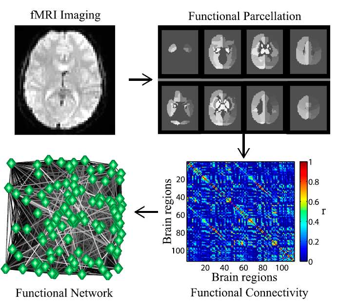
Figure 1: Multiple steps are needed to go from data acquisition to producing the finalfunctional brain graph, and each choice has effects on the final network. Once the methodof brain measurement has been chosen, the next step is to define the network nodes. In thecase of fMRI, this can be done using parcellation schemes. This is the delineation of the braininto parcels using a common approach or a set of criteria [9]. The association between nodesmust be calculated; with fMRI data this can be done by measuring the pairwise correlation inBOLD (Blood Oxygen Level-Dependent) signal. The resulting network can be presented ina weighted form or be thresholded to produce a binary matrix. This figure is from Ref. [17]and is used with permission.
this simplifies the adjacency matrix, it also results in a loss of information. The datasets used in this study have been thresholded and kept as weighted. Since the edgeswere defined through measuring correlation, the resulting matrices are symmetric,but there are ways of measuring the connectivity that results in a directed network,such as Granger causality and Bayes net methods [24].
The potential for the modality of the neuroscientific data, the experimental design,
preprocessing steps, and network construction to affect the resulting brain graphmeans that comparison between results from analysing brain graphs from differentdata sets must be treated with caution.[14]
The brain is a dynamic complex system that evolves over multiple time scales. Itexhibits phase-locked electromagnetic oscillations over a range of frequencies [5]. Toput the time scales into perspective, the firing of an action potential in a neuron takes
about 100ms, while plastic change in synaptic strength operates over time scales ofminutes to hours, and repair in cognitive function after brain damage occurs overa duration of years. It is therefore necessary to measure the dynamics of the brainover different time scales to gain a more complete understanding of the system. Anecessary prospect for brain graph analysis is to model how brain functional networktopology and geometry changes over time [4].
One method for investigating the time evolution of networks is to quantify how
community structure changes over time. Communities can be defined as groups ina network that contain nodes that are more densely connected amongst themselves,with sparser connections between groups. One way to estimate community structurein a network is through optimising a quality function. Although community struc-ture was initially applied to static networks, the methodology has been extended tofind community structure in time dependent and multiplex networks [18]. These arenetworks that consist of layers of adjacency matrices. In this case, the quality functionis optimised through considering interlayer and intralayer couplings between nodes.
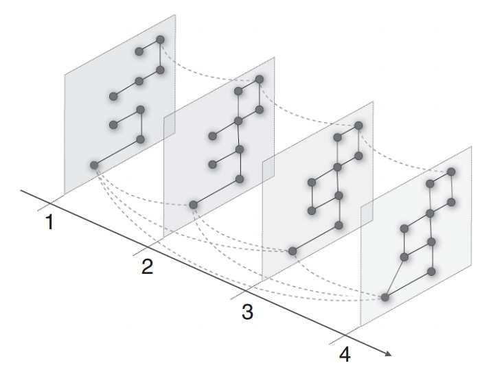
Intralayer couplings are connections between different nodes on the same networklayer. Interlayer couplings are those between the same node on different networklayers. The network layers can encode connections of a different type, of differentscales, or of different time points.
Figure 2: Community detection in multilayer networks. By introducing interlayer couplings,communities can be found that span network layers. The network layers can represent con-nections at different time points or of a different type. This figure is from Ref. [18] and isused with permission.
To quantify fluctuations in community structure in a network, a measure of flexi-
bility can be used. This can be defined as the number of times that each node changesallegiance to a community [17]. It has been found that flexibility of a brain graph
from fMRI scans is a predictor of human learning [17].
Background on the data sets
Cornell data set
The first data set I used for this report was provided by the lab of Dr. Nicholas Schiff,Cornell University. It contains correlation matrices from the time series of a BOLDsignal for 90 ROIs (regions of interest) from resting fMRI scans from 7 individuals, 5of whom were healthy and 2 of whom had brain damage. Each individual had imageacquisition taken at 2–4 different points in time, with some of the time intervals aslarge as a year. There are therefore 2–4 sets of correlation matrices per individual.
There were between 88–90 nodes in each correlation matrix. However, because com-parative network analysis is difficult for graphs containing different nodes, I usedonly the common ROIs (84 in total). Both patients regain some cognitive function intheir later respective time points [1].
Cambridge data set
The second data set came from the group of Ed Bullmore at the University of Cam-bridge. The data set consisted of BOLD fMRI time series data taken at 498 timepoints for 471 ROIs from 15 healthy individuals and from 12 patients diagnosed withschizophrenia [16]. There were 3 different time series for each individual correspond-ing to 3 types of medication: Aripiprazole, Sulpiride, or a placebo. Aripiprazole andSulpiride are anti-psychotic drugs.
The notion of flexibility suggests a hypothesis for the Cambridge data. Symptoms
of schizophrenia include difficulties in working and long-term memory, attention,executive functioning, and speed of processing. It could therefore be hypothesisedthat the brain graphs of Schizophrenic patients exhibit less flexibility.
The Core-periphery algorithm was applied to the Cornell data, although no mean-ingful result was found. The identification of a network into a core and peripheryis to define a densely connected mesoscale core, and a sparsely connected periphery,where the nodes in the core are also well connected to the periphery. A more detailedmethod can be found in Ref. [23].
Communicability and Spectral clustering on static networks
Communicability is a measure of information flow in a network. It takes into ac-count the transmission of information along the non-shortest paths as well as thegeodesics. It can also be seen as a way of quantifying the "connectedness" betweentwo nodes through the existence of shared neighbours, even if an edge between thethe two nodes does not exist [8]. Because the adjacency matrices used in this studyare weighted, I used a method that was adapted from the method for the binary case.
This is the method formulated by Crofts & Higham [6], which builds on a commu-nicability measure for binary adjacency networks by Estrada & Hatano [8]. In orderto derive a measure for communicability it is first useful to note that for a binaryadjacency matrix,
Ak� = the number of walks of length k between node i and j
where walks is defined as a traversal along edges in a network, and the length isdefined as the number of edges in the walk. This result is useful if we choose to seethe communicability between two nodes as a function of the number of walks lengthk = 1, 2, 3, etc. Estrada & Hatano noted that if one uses a penalisation factor of 1/k!for walks of length k, then the communicability between nodes i and j is
= �exp(A)� ,
where A is a binary adjacency matrix. The communicability matrix is defined asexp(A). Crofts & Higham noted that this function does not give the desired resultswhen applied to a weighted adjacency matrix. This is because a node with highconnectivity and weights can have a disproportionate influence on the resulting com-municability matrix. They therefore implemented a normalisation factor for each
edge Aij of
didj, where di = ∑ Aij is the strength of node i. The communicability
for a weighted network can then be defined as,
exp D− 12 AD− 12
where D is the N × N diagonal degree matrix D := diag(di). The resulting matrix
exp D− 12 AD− 12
gives a symmetric communicability network.
Once the communicability matrices have been defined, they can be partitioned withan unsupervised clustering algorithm such as spectral clustering method specified inthe paper by Higham et. al [13]. The output of the method groups the inputs based
on their similarity to each other. This method can also be applied to adjacency anddegree matrices, but Crofts & Higham suggest that the that communicability matrixgives the most effective results [7].
The first step is to use the communicability matrix to build a new matrix V so
that the communicability matrix data for each subject is formatted in columns. Forexample, if there were S communicability matrices containing M nodes, then thenew data matrix V would have S columns of length M(M − 1)/2 since an M × Mcommunicability matrix contains M(M − 1)/2 communicability weights. One canthen construct an S × S matrix of the form W = VTV, where Wij can be consideredthe similarity between network i and network j. The method proceeds by performingeigenvalue decomposition on the Laplacian of the weight matrix. The Laplacian isdefined as,
D − W,
D is an N × N diagonal matrix of the form ˜
D := diag( ˜
di) and ˜di := ∑ Wij. The
resulting Laplacian is a positive semi-definite matrix. When eigenvalue decomposi-
tion is performed on the Laplacian, the smallest eigenvalue is 0, with corresponding
eigenvector of 1, the vector where all elements are equal to 1. Assuming that the sec-
ond smallest eigenvalue is unique, the eigenvalues can be ordered in increasing order
as 0 = λ1 < λ2 < λ3 ≤ . ≤ λN with orthonormal eigenvectors v[1], v[2], ., v[N]. The
vector v[2] is known as the Fiedler vector. The Fiedler vector compresses the network
data for each individual into one dimension and has the potential to differentiate
between individuals. The sum of all components in the Fiedler vector must equal 1.
Time ordered community structure
Constructing a correlation matrix from time-series
The Cambridge data set consisted of time-series data. This can be consolidated intoadjacency networks that summarise the correlations between pairs of nodes over atime window ∆. The data is presented as a set values for N ROIs {X1, X2, ., XN} attime points {t1, t2, ., t f } and can be converted into a set of correlation matrices bymeasuring the relative similarity of pairs of nodes at mutual time points over a timewindow ∆ = [t1, t f ]. The method used is adapted from the method used in [21]. TheROIs in the data set yield the nodes in the final adjacency matrix. Defining Xi(t) asthe signal of ROI i at time t, one constructs for each time window of width ∆ thematrix component
Bij(t) = ∑ Xi(τ)Xj(τ).
Implementing a normalisation factor gives an adjacency matrix with component
Rij(t) =
This produces a symmetric correlation matrix with elements lying in the interval [-1,1]. The Cambridge data set contains 471 ROIs with BOLD signal measured at 498time points. The values chosen for ∆ in the study are 10, 20, 25, 30, and 40. None ofthese values are factors of 498, and so some of the data points were not used whenconstructing the adjacency matrices. For example, for ∆ = 10 there are 49 adjacencymatrices with 8 data points remaining that are not used.
Constructing a brain graph from correlation matrix
The values in the correlation matrix may not represent statistically significant func-tional relationships. To find the significant correlations, I followed the method fromRef. [17]. This involved calculating the p-value Pij for each element in the correlationmatrix Rij using the corrcoef function in MATLAB. I then tested p-values for signif-icance using a false discovery rate (FDR) [11] of p < 0.05. Any elements in Pij thatdid not pass the FDR threshold would have the corresponding value in Rij set to 0,and the resulting matrix was set to be the adjacency matrix A.
Before we consider communities in multilayer networks, we begin by consideringmodularity in static networks. The quality function Q for the partitioning of nodesinto communities is defined as [18],
ij − Zij
where δ(gi, gj) = 1 if nodes i and j are assigned to the same community, and 0otherwise. 2m is the number of ends of edges in the entire network. Zij is theexpected connection strength between nodes i and j under a null model. A commonmeasure for the null model is Zij = kikj/(2m), where ki = ∑j Aij. Zij is the expectedconnection strength between node i and j if the strength of each node in A is toremain the same but the connections between nodes are made at random [19]. Thisgives the Newman-Girvan model of modularity, defined as,
ij − 2m
To generalise equation (6) to multilayer networks of layers s = 1, 2, .T, the in-
terlayer couplings and the intralayer couplings must be considered. The intralayer
couplings between node i and j on layer s is defined as Aijs. The interlayer cou-pling that connects node j in layer r to itself in layer s is denoted as Cjrs [17]. Thegeneralised version of the modularity for multilayer networks is then,
Qmultilayer =
ijs − γ 2m
sr + δijCjsr
is, gjr),
where 2µ = ∑ijs Aij(s) + ∑srj Cjsr and is the sum of all of the edge weights in themultilayer network. The values gis , ms, and kis are generalisations of the parameters
gi, m, and ki in equation (6) to refer to a specific layer s. There is a new parameterγ, which is a resolution parameter that can have a different value for each layer but
in this study was a constant for all slices. It can be seen as γ = 1/t, where t isthe duration of a random walk across the network [15]. Small values of γ result inlarger communities and larger values of γ result in smaller communities. The choiceof γ = 1 is the default resolution for modularity. Cjsr can take the binary values of{0, ω}, and is a value of the strength of the coupling between interlayer links [18].
The GenLouvain algorithm
The generalized Louvain MATLAB code GenLouvain1.2 [18] was used to performcommunity detection. The algorithm was obtained from NetWiki, http://netwiki.
amath.unc.edu/GenLouvain/GenLouvain. This method is an adaption of the "Lou-vain" method, which is a greedy optimization method and returns high quality com-munity detection quickly [3].
The flexibility of a node can be defined as the number of times that a node changesallegiance to communities in successive time layers [2]. An alternative definition isto count how many different communities the node has belonged to. For example, anode that belongs to communities 1 and 2 in successive layers in the order "1, 2, 1, 2,1" has flexibility of 4 by the first definition and a flexibility of 2 by the second. Theflexibility of the entire network is then defined as the mean flexibility for all nodes.
For clarity we will call the first definition of flexibility flexibility 1 and the seconddefinition flexibility 2.
Spectral clustering on Cornell data
I constructed a communicability matrix for each subject from the Cornell data asgiven in equation (2). I then followed the spectral clustering procedure as specifiedin section 3.2.1 for the communicability and adjacency matrices. The Cornell dataset consisted of 21 subjects and 84 common nodes between them. The data matri-ces Vi contained either the communicability data or the adjacency data and had thedimensions of ((842 − 84)/2 = 3846) × 21.
Eigenvalue decomposition was performed on the Laplacian (eq. 3) and the result-
ing components from the Fiedler vector v[2] are shown in fig. (3). Spectral clustering
is partially successful at classifying healthy ('+') individuals and brain-damaged ('o')
individuals, but it does not appear to completely distinguish them, as one of the com-
ponents for a brain damaged subject in v[2] lies amongst the healthy subjects. The
method is also unable to show the improvement in cognitive ability for the brain-
damaged subjects. For an ideal result, the v[2] components for the later time points
from the Fiedler vector from brain-damaged subjects would be clustered near the
healthy individuals. It is also unclear why there is such a large jump between the
vector component values for individual 15 and 16.
The results from performing spectral clustering (section 3.2.1) on the adjacency
matrix is shown in fig. (4). It can been seen that the method was unsuccessful atdistinguishing between healthy and brain-damaged individuals. Crofts et. al havealso found that the communicability matrix works as a more successful input thanthe adjacency matrix when using the spectral clustering method used in this report[7].
Fieldler vector component
Figure 3: Components of the Fiedler vector v[2] after performing spectral clustering as specified in
Ref. [13] on communicability matrices from healthy and brain-damaged individuals. Brain-damaged
individuals are shown as 'o' and healthy individuals as '+'. The method is somewhat successful in
that it gives some distinction between healthy and brain-damaged. However this method fails to show
that the patients increased in their cognitive ability at later time points. Spectral clustering presents
one of the patients at time point 1 as being more similar to the healthy individuals
Fieldler vector components
Figure 4: Components of the Fiedler vector v[2] after performing spectral clustering as specified
in Ref. [13] on adjacency matrices from healthy and brain-damaged individuals. Brain-damaged
individuals are shown as 'o' and healthy individuals as '+'. Unlike spectral clustering for the commu-
nicability matrix, applying spectral clustering to the adjacency matrix does not distinguish between
healthy and brain-damaged individuals.
Community structure of time-series data
I converted the time-series data into adjacency matrices by using different time win-dows ∆ to measure the correlation between ROIs. Time windows were chosen of∆ =10, 20, 30, and 40 time points. I then ran the GenLouvain algorithm with parame-ters ω = 0.5 and γ = 0.5 and calculated the mean flexibility of the multiplex networkfor each patient and control on Aripiprazole, Sulpiride and placebo. Both definitionsof flexibility as defined in section 3.4.2 were used. I plot the results in fig.s (5) and(6). The results show that for both definitions of flexibility and for every choice of∆, the controls have a higher flexibility than the patients. What is unexpected is thatthe antipyschotic drugs do not seem to decrease the gap in difference of flexibilitybetween controls and patients. In fact, the largest difference in flexibility betweenpatient and control is with the drug Aripiprazole, and this is seen most clearly withthe second definition of flexibility (fig. (6)). It is interesting that controls taking Arip-iprazole have a higher flexibility than when they are on a placebo, while patients onAripiprazole show at certain values of ∆ (∆ = 20, 30 in fig. (5) and fig. (6)) have alower flexibility than when they are on a placebo.
Ariprazole − cAriprazole − pPlacebo − cPlacebo − p
Sulpiride − cSulpiride − p
Mean flexibility per node
Width of time window ∆
Figure 5: Mean flexibility (flexibility measure 1) per node from multilayer networks createdfrom time-series with time windows of width ∆ =10, 20, 30, 40. Patients and controls havebeen treated with the antipyschotic drugs Aripiprazole, Sulpiride or a placebo. It can be seenthat regardless of the choice of time window width ∆, the controls have a higher flexibilitythat the patients
Robustness of flexibility
I found the mean flexibility from one multiplex network over a range of values of γand ω in order to see how robust the value of flexibility is. The adjacency matriceswere constructed from the time-series data from a control taking a placebo and a timewindow of ∆ = 20 was used. It is important to check whether values of flexibilityare robust or are instead an artefact of the values of γ and ω. The values of ω usedwere in the range [0,1] and the values of γ used were in the range [0.5,10]. Thesewere found to be values that give a reasonable community structure, for example,γ was not so small as to have each node in an isolated community or too big as tohave communities that would span a network layer. Similarly, ω was large enoughto have some coupling between layers but not so large that all layers were groupedinto communities. I plot the results in fig. (7). It can be seen for both measures offlexibility that the value of flexibility is robust over all values of ω, while the measureflexibility 2 is not robust for γ ∈ [0.5, 4].
This explains why there is a large difference between the two measures of flexibil-
ity shown in fig. (5) and fig. (6)). I used the value of γ = 0.5 in community detection,
Ariprazole − cAriprazole − p
Placebo − cPlacebo − pSulpiride − c
No. of communities per node
Width of time window ∆
Figure 6: Mean flexibility (flexibility measure 2) per node from multilayer networks createdfrom time-series with time windows of width ∆ =10, 20, 30, 40. Patients and controls havebeen treated with the antipyschotic drugs Aripiprazole, Sulpiride or a placebo. It can be seenthat regardless of the choice of time window width ∆, the controls have a higher flexibilitythat the patientsIt can be seen that the difference in flexibility between patients and controlsis always greater with the drug Aripiprazole.
which we now know to be a value within which the second measure of flexibility isnot robust.
(a) flexibility measure 1
(b) flexibility measure 2
Figure 7: I tested the robustness of both measures of flexibility over a range of values ofγ and ω. These are parameters in the multilayer model of community detection [18]. Ichose values of γ and ω that gave reasonable community structure. It can be seen for bothmeasures of flexibility that the value of flexibility is robust over all chosen values of ω, whilethe measure flexibility 2 is not robust for γ ∈ [0.5, 4].
The results in Section 4 compare brain graphs from healthy versus unhealthy indi-viduals in order to attempt to distinguish patients from controls. This was moresuccessful with the Cambridge data because the data sets contained temporal infor-mation which allowed the more powerful tool of multilayer community detection tobe used. The Cornell data, by contrast, contained correlation matrices without timeseries data and there were at most 4 time points per individual. This was not suf-ficient to distinguish between patients from controls and most vitally show that thepatients regained some cognitive function at later time points. The measure of com-municability could only go as far as giving some distinction between brain-damagedand healthy individuals. What is more interesting to neuroscience would be to findmeasures that robustly characterise a brain graph and can be used to inform what ishappening in the physical system.
The was more scope for analysing the data with the Cambridge data set. Temporal
adjacency matrices were constructed from the time-series data and then communitydetection for multilayer networks was used to assign nodes to communities. I thenmeasured the flexibility of the nodes. Analysing time-series data opened up morecomplications, however, as many parameters were used in each step of the analysis- the length of time window ∆ for measuring the correlation between pairs of nodesand the values of ω and γ used in multilayer community detection. It is hard to saywhich regions of parameter space give the most accurate reflection of the subjectsundergoing fMRI scans. γ can be interpreted as the inverse time for a random walkacross the network, so there is some natural intuition for how γ affects communitydetection. The effects of ω are harder to discern. A value of ω = 0 means that thereis no coupling between the network layers. A value of ω = ∞ is the mean-fielddescription in which there is an average coupling between the same node over alllayers. What effects ω has on the network at values in between is less certain. Ideallya more thorough investigation on how the choice of ∆, γ and ω influences the resultsshould be conducted.
The results from the Cambridge data show that controls have a higher flexibility
than patients regardless of which medication they are on (Sulpiride, Aripiprazole, orplacebo). Additionally, the difference in flexibility between patients and controls wasconsistently larger for those on Aripiprazole compared to those taking Sulpiride ora Placebo. Aripiprazole has been prescribed to patients in the US for over 10 years[10], whereas Sulpiride is a comparatively newer drug. Sulpiride has been foundin studies to have fewer extrapyramidial side effects, such as dystonia, parkinson-ism, and akathisia, than older antipsychotic drugs [12]. The extrapyramidial systemis defined group of structures in the brain that are involved in motor function [20].
This is something to consider when analysing fMRI data from patients taking Arip-
iprazole. What could be useful when analysing such a data set like the one fromCambridge would be some accompanying documentation detailing any side effectsthat the subjects may be experiencing.
Further work
My work included only a preliminary look into how the choices of parameters ∆, γand ω affect the results. Future work should focus on this in order to discern whichresults are robust, rather than artefacts of the parameters used.
I conducted time ordered community detection on the Cambridge data by com-
paring time-dependent network layers taken from the same individual. Another ap-proach would be to consider couplings between individuals (a multiplex network).
If both the time dependent inter-individual and intra-individual couplings are in-cluded, then the community detection would have to be reformulated to deal withrank-4 tensors.
This report details an investigation on fMRI BOLD signal data from healthy andunhealthy individuals using network science. I found that temporal information wasnecessary for characterising the data, which is a consequence of the brain being adynamic system. Analysis of temporal data is more complicated than that on a staticnetwork, since there is more methodological choice and the parameter space in themethods used is large. Correlation matrices were constructed from the time seriesdata of time window width ∆, and the GenLouvain algorithm made use of parametersγ and ω that can vary from [0, ∞). More research is needed to clarify how the valuesof ∆, γ, and ω affect the brain graph analysis before any definitive conclusions canbe made. From the preliminary studies in this report it was found that the flexibilityof a network is a way of distinguishing between schizophrenic patients and controlsregardless of whether they are on an antipsychotic drug (Aripiprazole or Sulpiride)or a placebo.
Many thanks to Mason Porter and Sang Hoon Lee for invaluable guidance and sug-gestions. Also thanks to Sudhin Shah at Cornell for help in analysing the Cornelldata, and to the Nicholas D. Schiff lab for providing it. Thanks to Professor Bull-more's lab at Cambridge for their data set. I must also give credit to Peter J. Mucha
for the GenLouvain code on Netwiki, http://netwiki.amath.unc.edu/GenLouvain/GenLouvain, and to Puck Rombach for the Core-periphery code [23].
[1] S. Shah (private communication 29/08/12).
[2] D.S. Bassett, N.F. Wymbs, M.A. Porter, P.J. Mucha, J.M. Carlson, and S.T. Grafton.
Dynamic reconfiguration of human brain networks during learning. Proceedingsof the National Academy of Sciences, 108(18):7641–7646, 2011.
[3] V.D. Blondel, J.L. Guillaume, R. Lambiotte, and E. Lefebvre. Fast unfolding
of communities in large networks. Journal of Statistical Mechanics: Theory andExperiment, 2008(10):P10008, 2008.
[4] E. Bullmore and O. Sporns. Complex brain networks: graph theoretical analysis
of structural and functional systems. Nature Reviews Neuroscience, 10(3):186–198,2009.
[5] E.T. Bullmore and D.S. Bassett. Brain graphs: graphical models of the human
brain connectome. Annual review of clinical psychology, 7:113–140, 2011.
[6] J.J. Crofts and D.J. Higham. A weighted communicability measure applied to
complex brain networks. Journal of The Royal Society Interface, 6(33):411–414, 2009.
[7] JJ Crofts, DJ Higham, R. Bosnell, S. Jbabdi, PM Matthews, TEJ Behrens, and
H. Johansen-Berg. Network analysis detects changes in the contralesional hemi-sphere following stroke. NeuroImage, 54(1):161–169, 2011.
[8] E. Estrada and N. Hatano. Communicability in complex networks. Physical
Review E, 77(3):036111, 2008.
[9] G. Flandin, F. Kherif, X. Pennec, D. Rivière, N. Ayache, and J.B. Poline. Parcel-
lation of brain images with anatomical and functional constraints for fmri dataanalysis. In Biomedical Imaging, 2002. Proceedings. 2002 IEEE International Sympo-sium on, pages 907–910. IEEE, 2002.
[10] U.S. Food and Drug Administration. http://www.fda.gov/Safety/MedWatch/
[11] C.R. Genovese, N.A. Lazar, and T. Nichols. Thresholding of statistical maps in
functional neuroimaging using the false discovery rate. NeuroImage, 15(4):870–878, 2002.
[12] J. Gerlach, K. Behnke, J. Heltberg, E. Munk-Anderson, and H. Nielsen. Sulpiride
and haloperidol in schizophrenia: a double-blind cross-over study of therapeuticeffect, side effects and plasma concentrations. The British Journal of Psychiatry,147(3):283–288, 1985.
[13] D.J. Higham, G. Kalna, and M. Kibble. Spectral clustering and its use in bioin-
formatics. Journal of computational and applied mathematics, 204(1):25–37, 2007.
[14] B. Horwitz. The elusive concept of brain connectivity. NeuroImage, 19(2):466–470,
[15] R. Lambiotte, J.C. Delvenne, and M. Barahona. Laplacian dynamics and multi-
scale modular structure in networks. Arxiv preprint arXiv:0812.1770, 2008.
[16] M.E. Lynall, D.S. Bassett, R. Kerwin, P.J. McKenna, M. Kitzbichler, U. Muller,
and E. Bullmore. Functional connectivity and brain networks in schizophrenia.
The Journal of Neuroscience, 30(28):9477–9487, 2010.
[17] A.V. Mantzaris, D.S. Bassett, N.F. Wymbs, E. Estrada, M.A. Porter, P.J. Mucha,
S.T. Grafton, and D.J. Higham. Dynamic network centrality summarizes learningin the human brain. Arxiv preprint arXiv:1207.5047, 2012.
[18] P.J. Mucha, T. Richardson, K. Macon, M.A. Porter, and J.P. Onnela. Commu-
nity structure in time-dependent, multiscale, and multiplex networks. Science,328(5980):876–878, 2010.
[19] M. Newman. Networks: an Introduction. Oxford University Press, Inc., 2010.
[20] BrainInfo University of Washington. http://braininfo.rprc.washington.edu/
[21] T. Prescott. Examining dynamic network structures in relation to the spread
of infectious diseases,
[22] Human Connectome Project. http://www.humanconnectomeproject.org/.
[23] M.P. Rombach, M.A. Porter, J.H. Fowler, and P.J. Mucha. Core-periphery struc-
ture in networks. arXiv preprint arXiv:1202.2684, 2012.
[24] S.M. Smith, K.L. Miller, G. Salimi-Khorshidi, M. Webster, C.F. Beckmann, T.E.
Nichols, J.D. Ramsey, and M.W. Woolrich. Network modelling methods for fmri.
NeuroImage, 54(2):875–891, 2011.
[25] R.W. Williams and K. Herrup. The control of neuron number. Annual Review of
Neuroscience, 11(1):423–453, 1988.
Source: https://people.maths.ox.ac.uk/porterm/research/lever_report-final_sysbio.pdf
Die Zeitschrift der Ärztinnen und Ärzte Management von Notfällen und Blutungen Autoren: Univ.-Prof. Dr. Marianne Brodmann, Priv.-Doz. Dr. Benjamin Dieplinger, Univ.-Prof. Dr. Hans Domanovits, Univ.-Prof. Dr. Sabine Eichinger-Hasenauer, Univ.-Prof. Dr. Dietmar Fries, Prim. Univ.-Prof. Dr. Reinhold Függer, OA Dr. Manfred Gütl, Univ.-Doz. Dr. Hans-Peter Haring, Univ.-Prof. Dr. Michael Hiesmayr, Univ.-Prof. Dr. Paul A. Kyrle, Prim. Univ.-Prof. Dr. Wilfried Lang, Univ.-Doz. Dr. Stefan Marlovits, Univ.-Prof. Dr. Erich Minar, OA Dr. Peter Perger, Univ.-Prof. Dr. Peter Quehenberger, Univ.-Prof. Dr. Martin Schillinger, Priv.-Doz. Dr. Barbara Steinlechner, OA Dr. Wolfgang Sturm.
‘Reflection' Gold Show Garden call of the wild A sophisticated palette with wispy grasses, including Panicum ‘Heavy Metal' and P. virgatum, creates a carefully orchestrated wild and casual planting style for this design. Silver and white, with accents of pink and yellow, contrasts with the boathouse, which is clad with Oregon timber that has been burned to create